수치입력 수치예측 모델 레시피
수치를 입력해서 수치를 예측하는 모델들에 대해서 알아보겠습니다. 수치예측을 위한 데이터셋 생성을 해보고, 선형회귀를 위한 가장 간단한 퍼셉트론 신경망 모델부터 깊은 다층퍼셉트론 신경망 모델까지 구성 및 학습을 시켜보겠습니다
데이터셋 준비
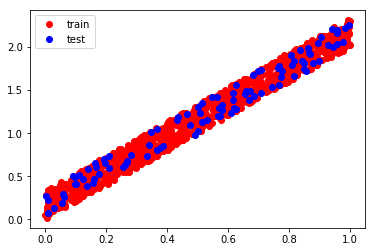
입력 x에 대해 2를 곱해 두 배 정도 값을 갖는 출력 y가 되도록 데이터셋을 생성해봤습니다. 선형회귀 모델을 사용한다면 Y = w * X + b 일 때, w가 2에 가깝고, b가 0.16에 가깝게 되도록 학습시키는 것이 목표입니다.
import numpy as np

# 데이터셋 생성
x_train = np.random.random((1000, 1))
y_train = x_train * 2 + np.random.random((1000, 1)) / 3.0
x_test = np.random.random((100, 1))
y_test = x_test * 2 + np.random.random((100, 1)) / 3.0

# 데이터셋 확인
%matplotlib inline
import matplotlib.pyplot as plt

plt.plot(x_train, y_train, 'ro')
plt.plot(x_test, y_test, 'bo')
plt.legend(['train', 'test'], loc='upper left')
plt.show()
레이어 준비
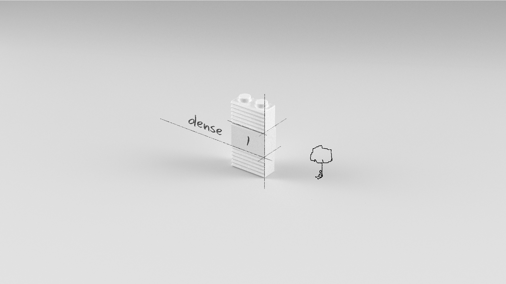
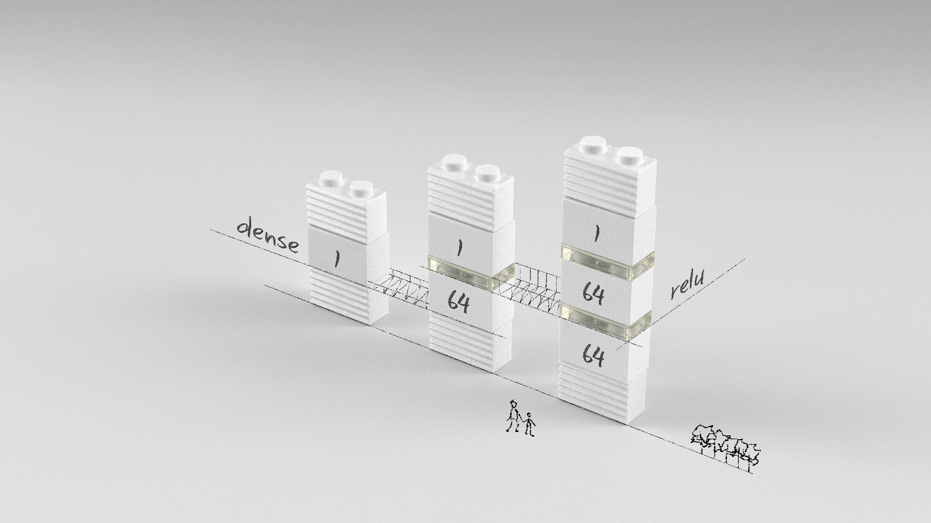
본 장에서 사용되는 블록들은 다음과 같습니다.
| 블록 | 이름 | 설명 |
|---|---|---|
 |
Input data, Labels | 1차원의 입력 데이터 및 라벨입니다. |
 |
Dense | 모든 입력 뉴런과 출력 뉴런을 연결하는 전결합층입니다. |
 |
relu | 활성화 함수로 주로 은닉층에 사용됩니다. |
모델 준비
수치예측을 하기 위해 선형회귀 모델, 퍼셉트론 신경망 모델, 다층퍼셉트론 신경망 모델, 깊은 다층퍼셉트론 신경망 모델을 준비했습니다.
선형회귀 모델
가장 간단한 1차 선형회귀 모델로 수치예측을 해보겠습니다. 아래 식에서 x, y는 우리가 만든 데이터셋이고, 회귀분석을 통해서, w와 b값을 구하는 것이 목표입니다.
Y = w * X + b
w와 b값을 구하게 되면, 임의의 입력 x에 대해서 출력 y가 나오는 데 이것이 예측 값입니다. w, b 값은 분산, 공분산, 평균을 이용하여 쉽게 구할 수 있습니다.
w = np.cov(X, Y, bias=1)[0,1] / np.var(X)
b = np.average(Y) - w * np.average(X)
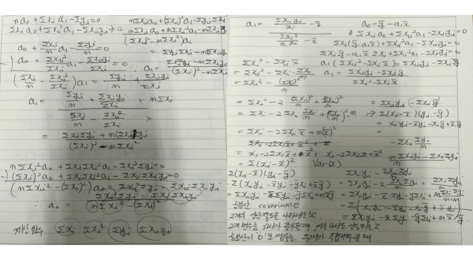
간단한 수식이지만 이 수식을 도출하기란 꽤나 복잡습니다. 오차를 최소화하는 극대값을 구하기 위해 편미분을 수행하고, 다시 식을 전개하는 등등의 과정이 필요합니다.
퍼셉트론 신경망 모델
Dense 레이어가 하나이고, 뉴런의 수도 하나인 가장 기본적인 퍼셉트론 모델입니다. 즉 웨이트(w) 하나, 바이어스(b) 하나로 전형적인 Y = w * X + b를 풀기 위한 모델입니다. 수치 예측을 하기 위해서 출력 레이어에 별도의 활성화 함수를 사용하지 않았습니다. w, b 값이 손으로 푼 선형회귀 최적해에 근접하려면 경우에 따라 만번이상의 에포크가 필요합니다. 실제로 사용하지는 않는 모델이지만 선형회귀부터 공부하시는 분들에게는 입문 모델로 나쁘지 않습니다.
model = Sequential()
model.add(Dense(1, input_dim=1))
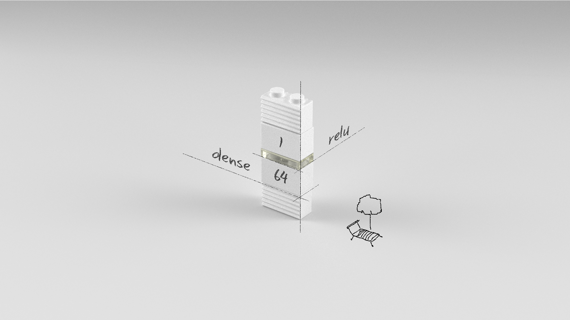
다층퍼셉트론 신경망 모델
Dense 레이어가 두 개인 다층퍼셉트론 모델입니다. 첫 번째 레이어는 64개의 뉴런을 가진 Dense 레이어이고 오류역전파가 용이한 relu 활성화 함수를 사용하였습니다. 출력 레이어인 두 번째 레이어는 하나의 수치값을 예측을 하기 위해서 1개의 뉴런을 가지며, 별도의 활성화 함수를 사용하지 않았습니다.
model = Sequential()
model.add(Dense(64, input_dim=1, activation='relu'))
model.add(Dense(1))
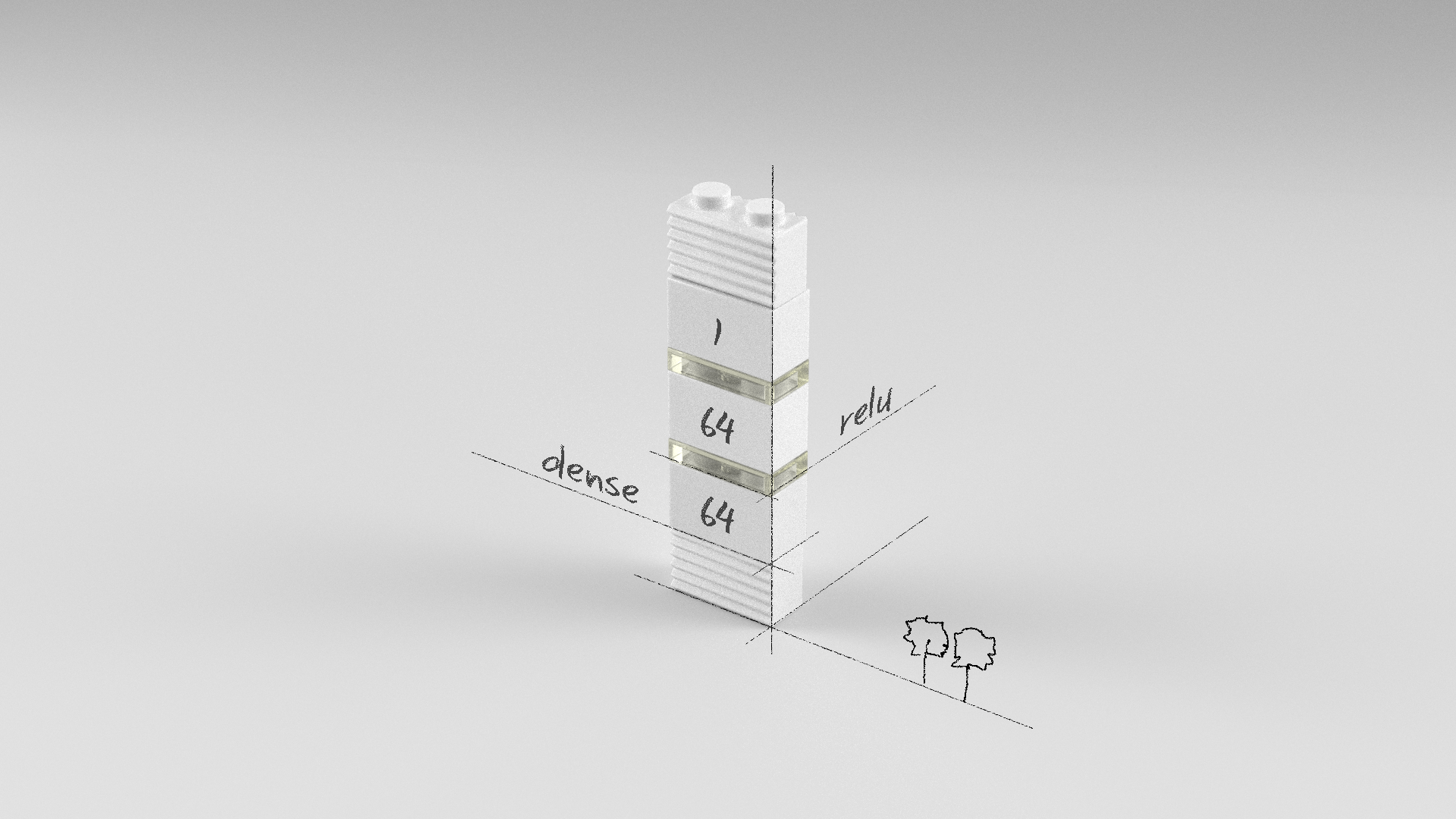
깊은 다층퍼셉트론 신경망 모델
Dense 레이어가 총 세 개인 다층퍼셉트론 모델입니다. 첫 번째, 두 번째 레이어는 64개의 뉴런을 가진 Dense 레이어이고 오류역전파가 용이한 relu 활성화 함수를 사용하였습니다. 출력 레이어인 세 번째 레이어는 하나의 수치값을 예측을 하기 위해서 1개의 뉴런을 가지며, 별도의 활성화 함수를 사용하지 않았습니다.
model = Sequential()
model.add(Dense(64, input_dim=1, activation='relu'))
model.add(Dense(64, activation='relu'))
model.add(Dense(1))
전체 소스
앞서 살펴본 선형회귀 모델, 퍼셉트론 신경망 모델, 다층퍼셉트론 신경망 모델, 깊은 다층퍼셉트론 신경망 모델의 전체 소스는 다음과 같습니다.
선형회귀 모델
# 0. 사용할 패키지 불러오기
import numpy as np
from sklearn.metrics import mean_squared_error
import random

# 1. 데이터셋 생성하기
x_train = np.random.random((1000, 1))
y_train = x_train * 2 + np.random.random((1000, 1)) / 3.0
x_test = np.random.random((100, 1))
y_test = x_test * 2 + np.random.random((100, 1)) / 3.0

x_train = x_train.reshape(1000,)
y_train = y_train.reshape(1000,)
x_test = x_test.reshape(100,)
y_test = y_test.reshape(100,)

# 2. 모델 구성하기
w = np.cov(x_train, y_train, bias=1)[0,1] / np.var(x_train)
b = np.average(y_train) - w * np.average(x_train)

print w, b

# 3. 모델 평가하기
y_predict = w * x_test + b
mse = mean_squared_error(y_test, y_predict)
print('mse : ' + str(mse))
2.00574308629 0.166691995049
mse : 0.0103976035867
퍼셉트론 신경망 신경망 모델
# 0. 사용할 패키지 불러오기
import numpy as np
from keras.models import Sequential
from keras.layers import Dense
import random
# 1. 데이터셋 생성하기
x_train = np.random.random((1000, 1))
y_train = x_train * 2 + np.random.random((1000, 1)) / 3.0
x_test = np.random.random((100, 1))
y_test = x_test * 2 + np.random.random((100, 1)) / 3.0
# 2. 모델 구성하기
model = Sequential()
model.add(Dense(1, input_dim=1))
# 3. 모델 학습과정 설정하기
model.compile(optimizer='rmsprop', loss='mse')
# 4. 모델 학습시키기
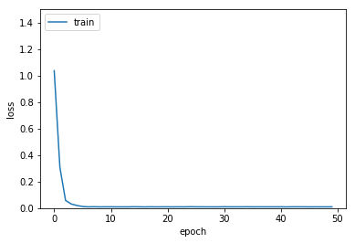
hist = model.fit(x_train, y_train, epochs=50, batch_size=64)
w, b = model.get_weights()
print w, b
# 5. 학습과정 살펴보기
%matplotlib inline
import matplotlib.pyplot as plt
plt.plot(hist.history['loss'])
plt.ylim(0.0, 1.5)
plt.ylabel('loss')
plt.xlabel('epoch')
plt.legend(['train'], loc='upper left')
plt.show()
# 6. 모델 평가하기
loss = model.evaluate(x_test, y_test, batch_size=32)
print('loss : ' + str(loss))
Epoch 1/50
1000/1000 [==============================] - 0s - loss: 3.3772
Epoch 2/50
1000/1000 [==============================] - 0s - loss: 3.2768
Epoch 3/50
1000/1000 [==============================] - 0s - loss: 3.1915
...
Epoch 48/50
1000/1000 [==============================] - 0s - loss: 0.6717
Epoch 49/50
1000/1000 [==============================] - 0s - loss: 0.6426
Epoch 50/50
1000/1000 [==============================] - 0s - loss: 0.6149
[[-0.1403431]] [ 0.79356796]
 32/100 [========>.....................] - ETA: 0sloss : 0.608838057518
다층퍼셉트론 신경망 모델
# 0. 사용할 패키지 불러오기
import numpy as np
from keras.models import Sequential
from keras.layers import Dense
import random

# 1. 데이터셋 생성하기
x_train = np.random.random((1000, 1))
y_train = x_train * 2 + np.random.random((1000, 1)) / 3.0
x_test = np.random.random((100, 1))
y_test = x_test * 2 + np.random.random((100, 1)) / 3.0

# 2. 모델 구성하기
model = Sequential()
model.add(Dense(64, input_dim=1, activation='relu'))
model.add(Dense(1))

# 3. 모델 학습과정 설정하기
model.compile(optimizer='rmsprop', loss='mse')

# 4. 모델 학습시키기
hist = model.fit(x_train, y_train, epochs=50, batch_size=64)

# 5. 학습과정 살펴보기
%matplotlib inline
import matplotlib.pyplot as plt

plt.plot(hist.history['loss'])
plt.ylim(0.0, 1.5)
plt.ylabel('loss')
plt.xlabel('epoch')
plt.legend(['train'], loc='upper left')
plt.show()

# 6. 모델 평가하기
loss = model.evaluate(x_test, y_test, batch_size=32)
print('loss : ' + str(loss))
Epoch 1/50
1000/1000 [==============================] - 0s - loss: 3.3772
Epoch 2/50
1000/1000 [==============================] - 0s - loss: 3.2768
Epoch 3/50
1000/1000 [==============================] - 0s - loss: 3.1915
...
Epoch 48/50
1000/1000 [==============================] - 0s - loss: 0.0096
Epoch 49/50
1000/1000 [==============================] - 0s - loss: 0.0096
Epoch 50/50
1000/1000 [==============================] - 0s - loss: 0.0097
 32/100 [========>.....................] - ETA: 3sloss : 0.00962571099401
깊은 다층퍼셉트론 신경망 모델
# 0. 사용할 패키지 불러오기
import numpy as np
from keras.models import Sequential
from keras.layers import Dense
import random

# 1. 데이터셋 생성하기
x_train = np.random.random((1000, 1))
y_train = x_train * 2 + np.random.random((1000, 1)) / 3.0
x_test = np.random.random((100, 1))
y_test = x_test * 2 + np.random.random((100, 1)) / 3.0

# 2. 모델 구성하기
model = Sequential()
model.add(Dense(64, input_dim=1, activation='relu'))
model.add(Dense(64, activation='relu'))
model.add(Dense(1))

# 3. 모델 학습과정 설정하기
model.compile(optimizer='rmsprop', loss='mse')

# 4. 모델 학습시키기
hist = model.fit(x_train, y_train, epochs=50, batch_size=64)

# 5. 학습과정 살펴보기
%matplotlib inline
import matplotlib.pyplot as plt

plt.plot(hist.history['loss'])
plt.ylim(0.0, 1.5)
plt.ylabel('loss')
plt.xlabel('epoch')
plt.legend(['train'], loc='upper left')
plt.show()

# 6. 모델 평가하기
loss = model.evaluate(x_test, y_test, batch_size=32)
print('loss : ' + str(loss))
Epoch 1/50
1000/1000 [==============================] - 0s - loss: 3.3772
Epoch 2/50
1000/1000 [==============================] - 0s - loss: 3.2768
Epoch 3/50
1000/1000 [==============================] - 0s - loss: 3.1915
...
Epoch 48/50
1000/1000 [==============================] - 0s - loss: 0.0093
Epoch 49/50
1000/1000 [==============================] - 0s - loss: 0.0095
Epoch 50/50
1000/1000 [==============================] - ETA: 0s - loss: 0.008 - 0s - loss: 0.0094
 32/100 [========>.....................] - ETA: 4sloss : 0.0100720105693
학습결과 비교
퍼셉트론 신경망 모델 > 다층퍼셉트론 신경망 모델 > 깊은 다층퍼셉트론 신경망 모델 순으로 학습이 좀 더 빨리 되는 것을 확인할 수 있습니다.
| 퍼셉트론 신경망 모델 | 다층퍼셉트론 신경망 모델 | 깊은 다층퍼셉트론 신경망 모델 |
|---|---|---|
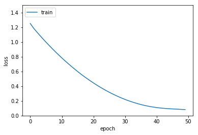 |
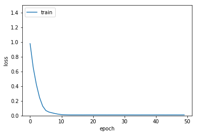 |
 |
요약
수치예측을 위한 퍼셉트론 신경망 모델, 다층퍼셉트론 신경망 모델, 깊은 다층퍼셉트론 신경망 모델을 살펴보고, 그 성능을 확인 해봤습니다.
같이 보기
- 강좌 목차
- 이전 : 순환 신경망 모델 만들어보기
- 다음 : 수치입력 이진분류 모델 레시피
책 소개
[추천사]
- 하용호님, 카카오 데이터사이언티스트 - 뜬구름같은 딥러닝 이론을 블록이라는 손에 잡히는 실체로 만져가며 알 수 있게 하고, 구현의 어려움은 케라스라는 시를 읽듯이 읽어내려 갈 수 있는 라이브러리로 풀어준다.
- 이부일님, (주)인사아트마이닝 대표 - 여행에서도 좋은 가이드가 있으면 여행지에 대한 깊은 이해로 여행이 풍성해지듯이 이 책은 딥러닝이라는 분야를 여행할 사람들에 가장 훌륭한 가이드가 되리라고 자부할 수 있다. 이 책을 통하여 딥러닝에 대해 보지 못했던 것들이 보이고, 듣지 못했던 것들이 들리고, 말하지 못했던 것들이 말해지는 경험을 하게 될 것이다.
- 이활석님, 네이버 클로바팀 - 레고 블럭에 비유하여 누구나 이해할 수 있게 쉽게 설명해 놓은 이 책은 딥러닝의 입문 도서로서 제 역할을 다 하리라 믿습니다.
- 김진중님, 야놀자 Head of STL - 복잡했던 머릿속이 맑고 깨끗해지는 효과가 있습니다.
- 이태영님, 신한은행 디지털 전략부 AI LAB - 기존의 텐서플로우를 활용했던 분들에게 바라볼 수 있는 관점의 전환점을 줄 수 있는 Mild Stone과 같은 책이다.
- 전태균님, 쎄트렉아이 - 케라스의 특징인 단순함, 확장성, 재사용성을 눈으로 쉽게 보여주기 위해 친절하게 정리된 내용이라 생각합니다.
- 유재준님, 카이스트 - 바로 적용해보고 싶지만 어디부터 시작할지 모를 때 최선의 선택입니다.