문장(시계열수치)입력 다중클래스분류 모델 레시피
문장을 입력해서 다중클래스를 분류하는 모델에 대해서 알아보겠습니다. 다중클래스 분류를 위한 데이터셋에 대해서 살펴보고 여러가지 다중클래스 분류 모델을 구성해보겠습니다. 이 모델들은 문장 혹은 시계열수치로 타입을 분류하는 문제를 풀 수 있습니다.
데이터셋 준비
로이터에서 제공하는 뉴스와이어 데이터셋을 이용하겠습니다. 이 데이터셋은 총 11,228개의 샘플로 구성되어 있습니다. 라벨은 46개 주제로 지정되어 0에서 45의 값을 가지고 있습니다. 케라스에서 제공하는 reuters의 load_data() 함수을 이용하면 데이터셋을 쉽게 얻을 수 있습니다. 데이터셋은 이미 정수로 인코딩되어 있으며, 정수값은 단어의 빈도수를 나타냅니다. 모든 단어를 고려할 수 없으므로 빈도수가 높은 단어를 위주로 데이터셋을 생성합니다. 15,000번째로 많이 사용하는 단어까지만 데이터셋으로 만들고 싶다면, num_words 인자에 15000이라고 지정하면 됩니다.
from keras.datasets import reuters
(x_train, y_train), (x_test, y_test) = reuters.load_data(num_words=15000)
훈련셋 8,982개와 시험셋 2,246개로 구성된 총 11,228개 샘플이 로딩이 됩니다. 훈련셋과 시험셋의 비율은 load_data() 함수의 test_split 인자로 조절 가능합니다. 각 샘플은 뉴스 한 건을 의미하며, 단어의 인덱스로 구성되어 있습니다. ‘num_words=20000’으로 지정했기 때문에 빈도수가 15,000을 넘는 단어는 로딩되지 않습니다. 훈련셋 8,982개 중 다시 7,000개을 훈련셋으로 나머지를 검증셋으로 분리합니다.
x_val = x_train[7000:]
y_val = y_train[7000:]
x_train = x_train[:7000]
y_train = y_train[:7000]
각 샘플의 길이가 달라서 모델의 입력으로 사용하기 위해 케라스에서 제공되는 전처리 함수인 sequence의 pad_sequences() 함수를 사용합니다. 이 함수는 두 가지 역할을 수행합니다.
- 문장의 길이를 maxlen 인자로 맞춰줍니다. 예를 들어 120으로 지정했다면 120보다 짧은 문장은 0으로 채워서 120단어로 맞춰주고 120보다 긴 문장은 120단어까지만 잘라냅니다.
- (num_samples, num_timesteps)으로 2차원의 numpy 배열로 만들어줍니다. maxlen을 120으로 지정하였다면, num_timesteps도 120이 됩니다.
from keras.preprocessing import sequence

x_train = sequence.pad_sequences(x_train, maxlen=120)
x_val = sequence.pad_sequences(x_val, maxlen=120)
x_test = sequence.pad_sequences(x_test, maxlen=120)
레이어 준비
앞 장의 “문장입력 이진분류 모델”에서 출력층의 활성화 함수만 다르므로 새롭게 소개되는 블록은 없습니다.
모델 준비
문장을 입력하여 다중클래스 분류를 하기 위해 다층퍼셉트론 신경망 모델, 순환 신경망 모델, 컨볼루션 신경망 모델, 순환 컨볼루션 신경망 모델을 준비했습니다.
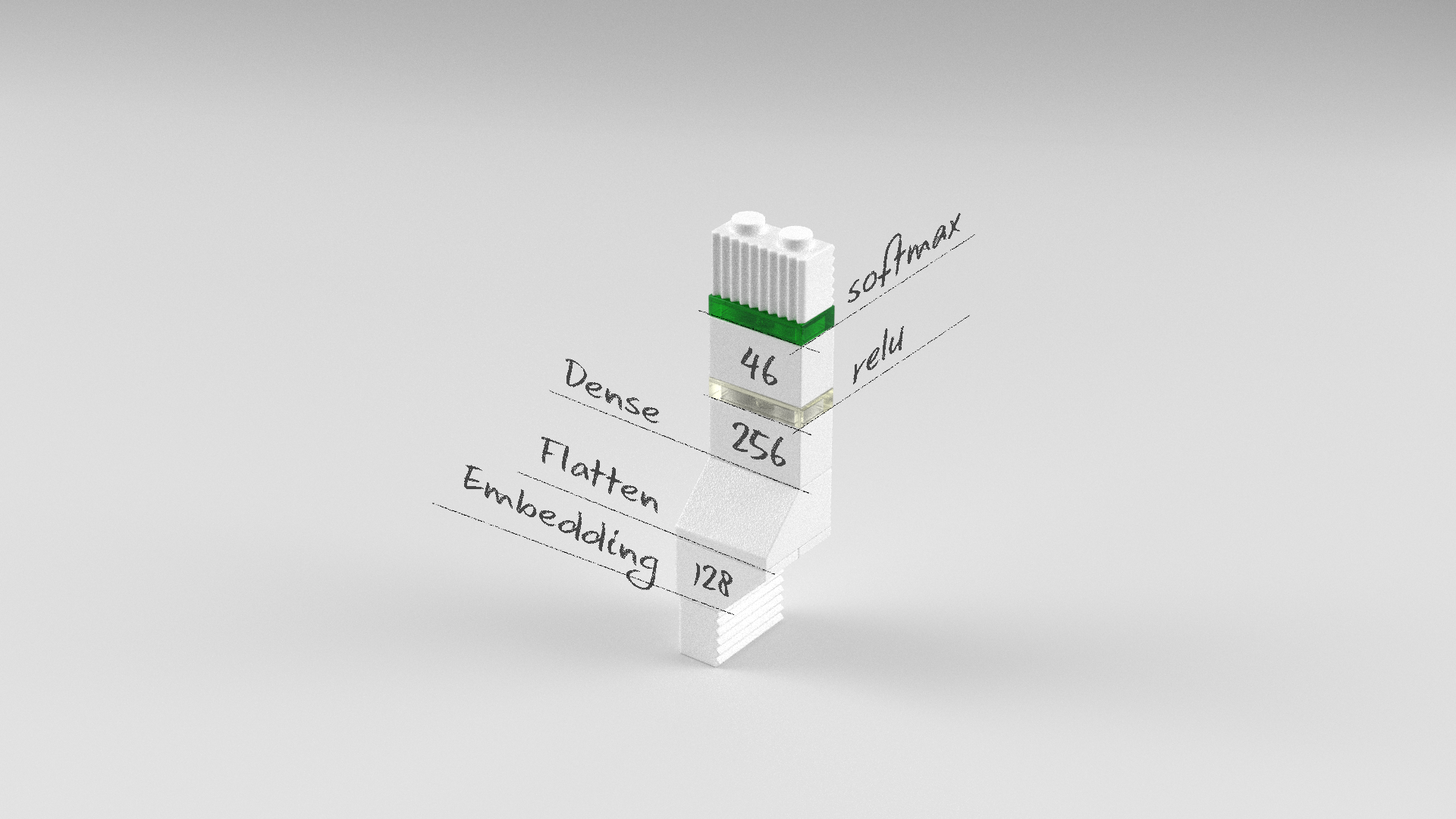
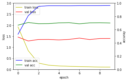
다층퍼셉트론 신경망 모델
임베딩 레이어는 0에서 45의 정수값으로 지정된 단어를 128벡터로 인코딩합니다. 문장의 길이가 120이므로 임베딩 레이어는 128 속성을 가진 벡터를 120개 반환합니다. 이를 플래튼 레이어를 통해 1차원 벡터로 만든 뒤 전결합층으로 전달합니다. 46개 주제를 분류해야 하므로 출력층의 활성화 함수로 ‘softmax’를 사용하였습니다.
model = Sequential()
model.add(Embedding(15000, 128, input_length=120))
model.add(Flatten())
model.add(Dense(256, activation='relu'))
model.add(Dense(46, activation='softmax'))
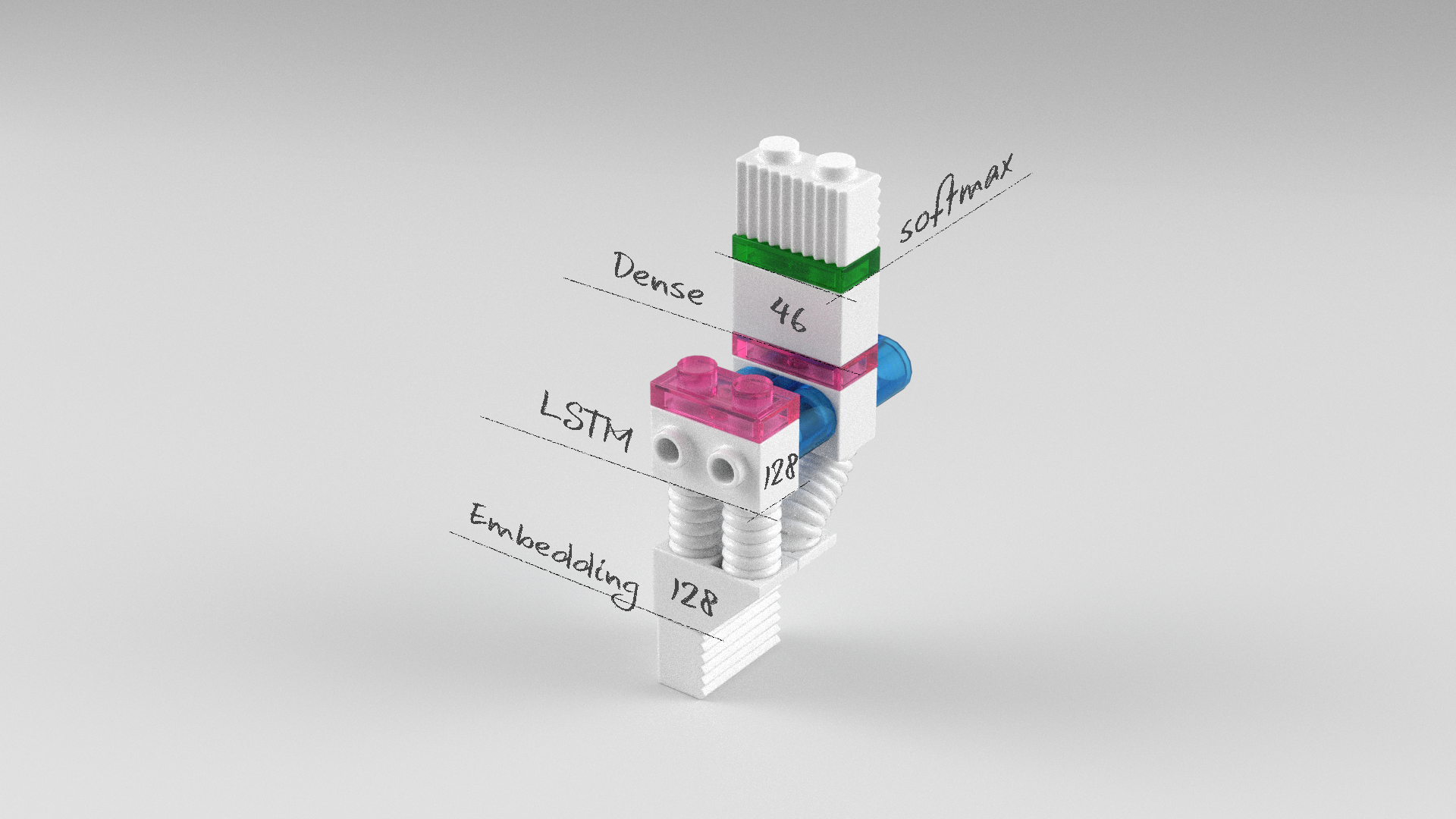
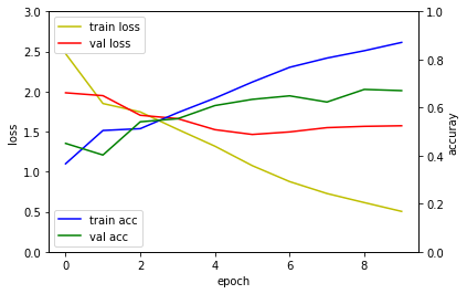
순환 신경망 모델
임베딩 레이어에서 반환되는 120개 벡터를 LSTM의 타입스텝으로 입력하는 모델입니다. LSTM의 input_dim은 임베딩 레이어에서 인코딩된 벡터크기인 128입니다.
model = Sequential()
model.add(Embedding(15000, 128))
model.add(LSTM(128))
model.add(Dense(46, activation='softmax'))
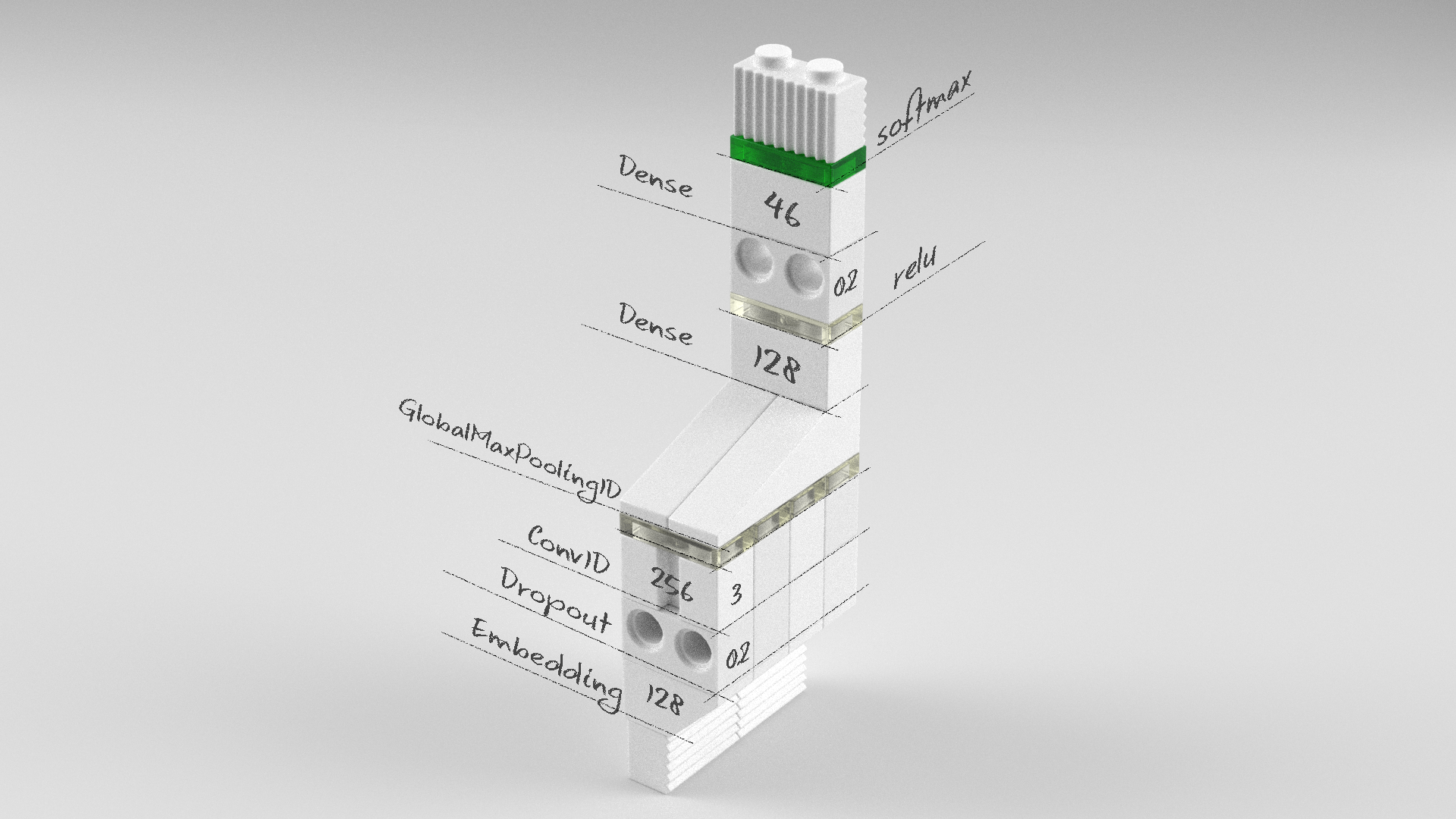
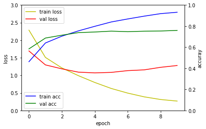
컨볼루션 신경망 모델
임베딩 레이어에서 반환되는 120개 벡터를 컨볼루션 필터를 적용한 모델입니다. 필터크기가 3인 컨볼루션 레이어는 120개의 벡터를 입력받아 118개의 벡터를 반환합니다. 벡터 크기는 컨볼루션 레이어를 통과하면서 128개에서 256개로 늘어났습니다. 글로벌 맥스풀링 레이어는 입력되는 118개 벡터 중 가장 큰 벡터 하나를 반환합니다. 그 벡터 하나를 전결합층을 통해서 다중클래스를 분류합니다.
model = Sequential()
model.add(Embedding(15000, 128, input_length=120))
model.add(Dropout(0.2))
model.add(Conv1D(256,
                 3,
                 padding='valid',
                 activation='relu',
                 strides=1))
model.add(GlobalMaxPooling1D())
model.add(Dense(128, activation='relu'))
model.add(Dropout(0.2))
model.add(Dense(46, activation='softmax'))
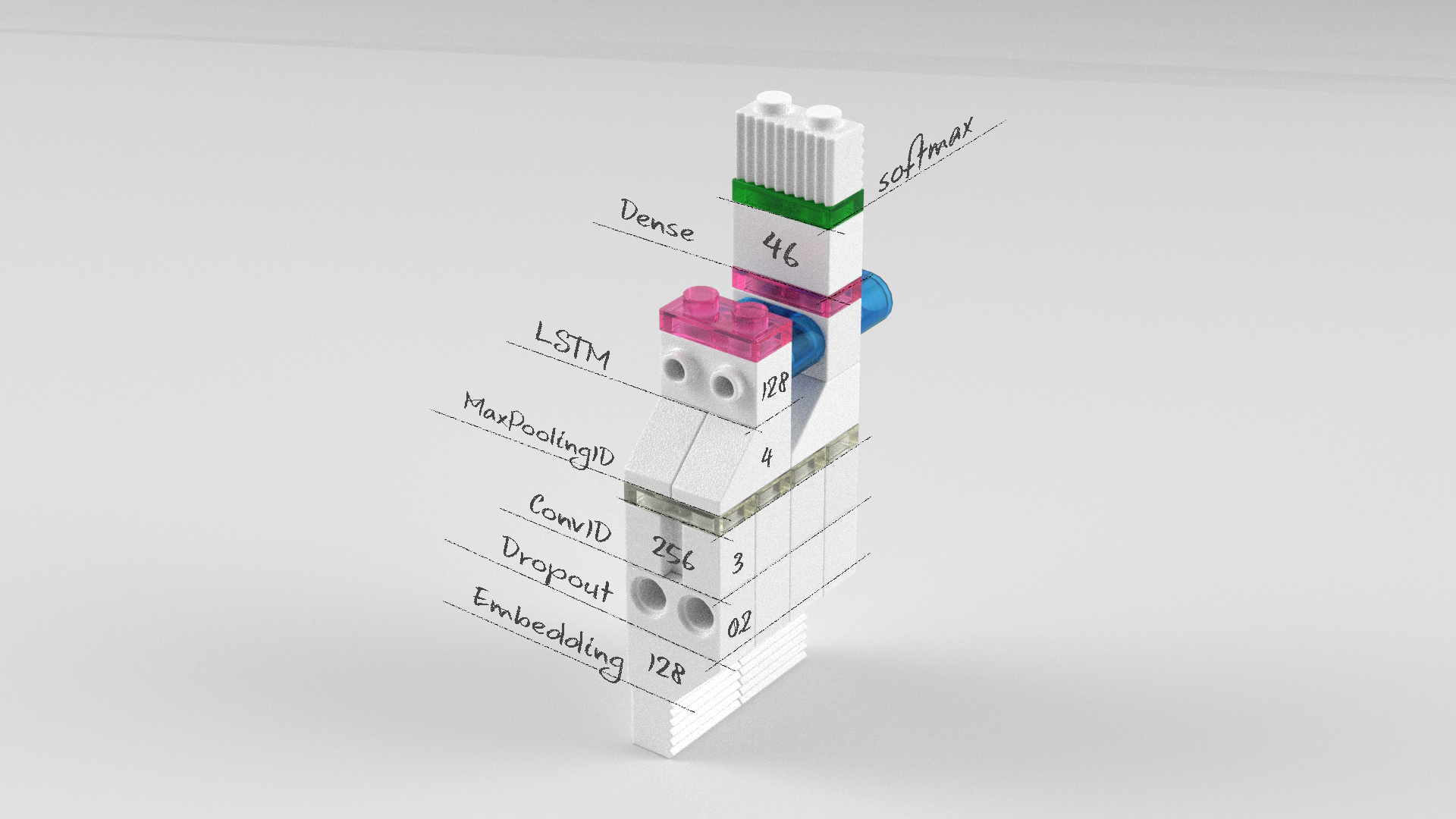
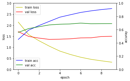
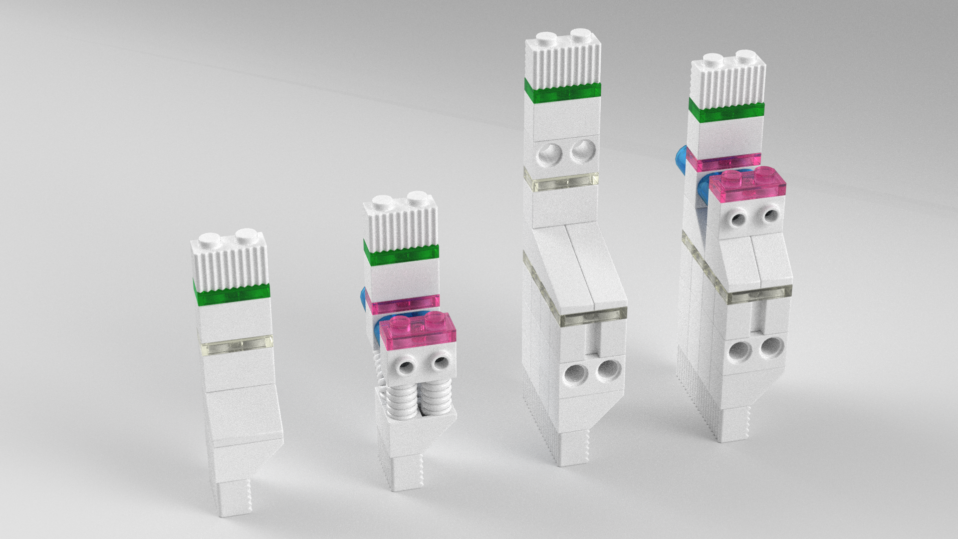
순환 컨볼루션 신경망 모델
컨볼루션 레이어에서 나온 특징벡터들을 맥스풀링를 통해 1/4로 줄여준 다음 LSTM의 입력으로 넣어주는 모델입니다. 컨볼루션 레이어에서 반환한 118개의 벡터를 1/4로 줄여서 29개를 반환합니다. 따라서 LSTM 레이어의 timesteps는 49개가 됩니다. 참고로 input_dim은 256입니다.
model = Sequential()
model.add(Embedding(max_features, 128, input_length=text_max_words))
model.add(Dropout(0.2))
model.add(Conv1D(256,
                 3,
                 padding='valid',
                 activation='relu',
                 strides=1))
model.add(MaxPooling1D(pool_size=4))
model.add(LSTM(128))
model.add(Dense(46, activation='softmax'))
전체 소스
앞서 살펴본 다층퍼셉트론 신경망 모델, 순환 신경망 모델, 컨볼루션 신경망 모델, 순환 컨볼루션 신경망 모델의 전체 소스는 다음과 같습니다.
다중퍼셉트론 신경망 모델
# 0. 사용할 패키지 불러오기
from keras.datasets import reuters
from keras.utils import np_utils
from keras.preprocessing import sequence
from keras.models import Sequential
from keras.layers import Dense, Embedding
from keras.layers import Flatten

max_features = 15000
text_max_words = 120

# 1. 데이터셋 생성하기

# 훈련셋과 시험셋 불러오기
(x_train, y_train), (x_test, y_test) = reuters.load_data(num_words=max_features)

# 훈련셋과 검증셋 분리
x_val = x_train[7000:]
y_val = y_train[7000:]
x_train = x_train[:7000]
y_train = y_train[:7000]

# 데이터셋 전처리 : 문장 길이 맞추기
x_train = sequence.pad_sequences(x_train, maxlen=text_max_words)
x_val = sequence.pad_sequences(x_val, maxlen=text_max_words)
x_test = sequence.pad_sequences(x_test, maxlen=text_max_words)

# one-hot 인코딩
y_train = np_utils.to_categorical(y_train)
y_val = np_utils.to_categorical(y_val)
y_test = np_utils.to_categorical(y_test)

# 2. 모델 구성하기
model = Sequential()
model.add(Embedding(max_features, 128, input_length=text_max_words))
model.add(Flatten())
model.add(Dense(256, activation='relu'))
model.add(Dense(46, activation='softmax'))

# 3. 모델 학습과정 설정하기
model.compile(loss='categorical_crossentropy', optimizer='adam', metrics=['accuracy'])

# 4. 모델 학습시키기
hist = model.fit(x_train, y_train, epochs=10, batch_size=64, validation_data=(x_val, y_val))

# 5. 학습과정 살펴보기
%matplotlib inline
import matplotlib.pyplot as plt

fig, loss_ax = plt.subplots()

acc_ax = loss_ax.twinx()

loss_ax.plot(hist.history['loss'], 'y', label='train loss')
loss_ax.plot(hist.history['val_loss'], 'r', label='val loss')
loss_ax.set_ylim([0.0, 3.0])

acc_ax.plot(hist.history['acc'], 'b', label='train acc')
acc_ax.plot(hist.history['val_acc'], 'g', label='val acc')
acc_ax.set_ylim([0.0, 1.0])

loss_ax.set_xlabel('epoch')
loss_ax.set_ylabel('loss')
acc_ax.set_ylabel('accuray')

loss_ax.legend(loc='upper left')
acc_ax.legend(loc='lower left')

plt.show()

# 6. 모델 평가하기
loss_and_metrics = model.evaluate(x_test, y_test, batch_size=64)
print('## evaluation loss and_metrics ##')
print(loss_and_metrics)
Train on 7000 samples, validate on 1982 samples
Epoch 1/10
7000/7000 [==============================] - 5s - loss: 1.9268 - acc: 0.5294 - val_loss: 1.4634 - val_acc: 0.6680
Epoch 2/10
7000/7000 [==============================] - 5s - loss: 0.8478 - acc: 0.8100 - val_loss: 1.2864 - val_acc: 0.7079
Epoch 3/10
7000/7000 [==============================] - 5s - loss: 0.2852 - acc: 0.9509 - val_loss: 1.3537 - val_acc: 0.6897
...
Epoch 8/10
7000/7000 [==============================] - 5s - loss: 0.1166 - acc: 0.9627 - val_loss: 1.3509 - val_acc: 0.7023
Epoch 9/10
7000/7000 [==============================] - 5s - loss: 0.1038 - acc: 0.9630 - val_loss: 1.3978 - val_acc: 0.7043
Epoch 10/10
7000/7000 [==============================] - 5s - loss: 0.1020 - acc: 0.9647 - val_loss: 1.3995 - val_acc: 0.7003

1600/2246 [====================>.........] - ETA: 0s## evaluation loss and_metrics ##
[1.4420637417773743, 0.68788958147818347]
순환 신경망 모델
# 0. 사용할 패키지 불러오기
from keras.datasets import reuters
from keras.utils import np_utils
from keras.preprocessing import sequence
from keras.models import Sequential
from keras.layers import Dense, Embedding, LSTM
from keras.layers import Flatten

max_features = 15000
text_max_words = 120

# 1. 데이터셋 생성하기

# 훈련셋과 시험셋 불러오기
(x_train, y_train), (x_test, y_test) = reuters.load_data(num_words=max_features)

# 훈련셋과 검증셋 분리
x_val = x_train[7000:]
y_val = y_train[7000:]
x_train = x_train[:7000]
y_train = y_train[:7000]

# 데이터셋 전처리 : 문장 길이 맞추기
x_train = sequence.pad_sequences(x_train, maxlen=text_max_words)
x_val = sequence.pad_sequences(x_val, maxlen=text_max_words)
x_test = sequence.pad_sequences(x_test, maxlen=text_max_words)

# one-hot 인코딩
y_train = np_utils.to_categorical(y_train)
y_val = np_utils.to_categorical(y_val)
y_test = np_utils.to_categorical(y_test)

# 2. 모델 구성하기
model = Sequential()
model.add(Embedding(max_features, 128))
model.add(LSTM(128))
model.add(Dense(46, activation='softmax'))

# 3. 모델 학습과정 설정하기
model.compile(loss='categorical_crossentropy', optimizer='adam', metrics=['accuracy'])

# 4. 모델 학습시키기
hist = model.fit(x_train, y_train, epochs=10, batch_size=64, validation_data=(x_val, y_val))

# 5. 학습과정 살펴보기
%matplotlib inline
import matplotlib.pyplot as plt

fig, loss_ax = plt.subplots()

acc_ax = loss_ax.twinx()

loss_ax.plot(hist.history['loss'], 'y', label='train loss')
loss_ax.plot(hist.history['val_loss'], 'r', label='val loss')
loss_ax.set_ylim([0.0, 3.0])

acc_ax.plot(hist.history['acc'], 'b', label='train acc')
acc_ax.plot(hist.history['val_acc'], 'g', label='val acc')
acc_ax.set_ylim([0.0, 1.0])

loss_ax.set_xlabel('epoch')
loss_ax.set_ylabel('loss')
acc_ax.set_ylabel('accuray')

loss_ax.legend(loc='upper left')
acc_ax.legend(loc='lower left')

plt.show()

# 6. 모델 평가하기
loss_and_metrics = model.evaluate(x_test, y_test, batch_size=64)
print('## evaluation loss and_metrics ##')
print(loss_and_metrics)
Train on 7000 samples, validate on 1982 samples
Epoch 1/10
7000/7000 [==============================] - 5s - loss: 1.9268 - acc: 0.5294 - val_loss: 1.4634 - val_acc: 0.6680
Epoch 2/10
7000/7000 [==============================] - 5s - loss: 0.8478 - acc: 0.8100 - val_loss: 1.2864 - val_acc: 0.7079
Epoch 3/10
7000/7000 [==============================] - 5s - loss: 0.2852 - acc: 0.9509 - val_loss: 1.3537 - val_acc: 0.6897
...
Epoch 8/10
7000/7000 [==============================] - 30s - loss: 0.7274 - acc: 0.8060 - val_loss: 1.5494 - val_acc: 0.6231
Epoch 9/10
7000/7000 [==============================] - 30s - loss: 0.6143 - acc: 0.8366 - val_loss: 1.5657 - val_acc: 0.6756
Epoch 10/10
7000/7000 [==============================] - 30s - loss: 0.5041 - acc: 0.8711 - val_loss: 1.5731 - val_acc: 0.6705

2240/2246 [============================>.] - ETA: 0s## evaluation loss and_metrics ##
[1.7008209377129164, 0.63980409619750878]
컨볼루션 신경망 모델
# 0. 사용할 패키지 불러오기
from keras.datasets import reuters
from keras.utils import np_utils
from keras.p`reprocessing import sequence
from keras.models import Sequential
from keras.layers import Dense, Embedding, LSTM
from keras.layers import Flatten, Dropout
from keras.layers import Conv1D, GlobalMaxPooling1D

max_features = 15000
text_max_words = 120

# 1. 데이터셋 생성하기

# 훈련셋과 시험셋 불러오기
(x_train, y_train), (x_test, y_test) = reuters.load_data(num_words=max_features)

# 훈련셋과 검증셋 분리
x_val = x_train[7000:]
y_val = y_train[7000:]
x_train = x_train[:7000]
y_train = y_train[:7000]

# 데이터셋 전처리 : 문장 길이 맞추기
x_train = sequence.pad_sequences(x_train, maxlen=text_max_words)
x_val = sequence.pad_sequences(x_val, maxlen=text_max_words)
x_test = sequence.pad_sequences(x_test, maxlen=text_max_words)

# one-hot 인코딩
y_train = np_utils.to_categorical(y_train)
y_val = np_utils.to_categorical(y_val)
y_test = np_utils.to_categorical(y_test)

# 2. 모델 구성하기
model = Sequential()
model.add(Embedding(max_features, 128, input_length=text_max_words))
model.add(Dropout(0.2))
model.add(Conv1D(256,
                 3,
                 padding='valid',
                 activation='relu',
                 strides=1))
model.add(GlobalMaxPooling1D())
model.add(Dense(128, activation='relu'))
model.add(Dropout(0.2))
model.add(Dense(46, activation='softmax'))

# 3. 모델 학습과정 설정하기
model.compile(loss='categorical_crossentropy', optimizer='adam', metrics=['accuracy'])

# 4. 모델 학습시키기
hist = model.fit(x_train, y_train, epochs=10, batch_size=64, validation_data=(x_val, y_val))

# 5. 학습과정 살펴보기
%matplotlib inline
import matplotlib.pyplot as plt

fig, loss_ax = plt.subplots()

acc_ax = loss_ax.twinx()

loss_ax.plot(hist.history['loss'], 'y', label='train loss')
loss_ax.plot(hist.history['val_loss'], 'r', label='val loss')
loss_ax.set_ylim([0.0, 3.0])

acc_ax.plot(hist.history['acc'], 'b', label='train acc')
acc_ax.plot(hist.history['val_acc'], 'g', label='val acc')
acc_ax.set_ylim([0.0, 1.0])

loss_ax.set_xlabel('epoch')
loss_ax.set_ylabel('loss')
acc_ax.set_ylabel('accuray')

loss_ax.legend(loc='upper left')
acc_ax.legend(loc='lower left')

plt.show()

# 6. 모델 평가하기
loss_and_metrics = model.evaluate(x_test, y_test, batch_size=64)
print('## evaluation loss and_metrics ##')
print(loss_and_metrics)
Train on 7000 samples, validate on 1982 samples
Epoch 1/10
7000/7000 [==============================] - 5s - loss: 1.9268 - acc: 0.5294 - val_loss: 1.4634 - val_acc: 0.6680
Epoch 2/10
7000/7000 [==============================] - 5s - loss: 0.8478 - acc: 0.8100 - val_loss: 1.2864 - val_acc: 0.7079
Epoch 3/10
7000/7000 [==============================] - 5s - loss: 0.2852 - acc: 0.9509 - val_loss: 1.3537 - val_acc: 0.6897
...
Epoch 8/10
7000/7000 [==============================] - 15s - loss: 0.3876 - acc: 0.8946 - val_loss: 1.1556 - val_acc: 0.7518
Epoch 9/10
7000/7000 [==============================] - 15s - loss: 0.3117 - acc: 0.9184 - val_loss: 1.2281 - val_acc: 0.7538
Epoch 10/10
7000/7000 [==============================] - 15s - loss: 0.2673 - acc: 0.9314 - val_loss: 1.2790 - val_acc: 0.7593

2240/2246 [============================>.] - ETA: 0s## evaluation loss and_metrics ##
[1.3962882223239672, 0.73107747111273791]
순환 컨볼루션 신경망 모델
# 0. 사용할 패키지 불러오기
from keras.datasets import reuters
from keras.utils import np_utils
from keras.preprocessing import sequence
from keras.models import Sequential
from keras.layers import Dense, Embedding, LSTM
from keras.layers import Flatten, Dropout
from keras.layers import Conv1D, MaxPooling1D

max_features = 15000
text_max_words = 120

# 1. 데이터셋 생성하기

# 훈련셋과 시험셋 불러오기
(x_train, y_train), (x_test, y_test) = reuters.load_data(num_words=max_features)

# 훈련셋과 검증셋 분리
x_val = x_train[7000:]
y_val = y_train[7000:]
x_train = x_train[:7000]
y_train = y_train[:7000]

# 데이터셋 전처리 : 문장 길이 맞추기
x_train = sequence.pad_sequences(x_train, maxlen=text_max_words)
x_val = sequence.pad_sequences(x_val, maxlen=text_max_words)
x_test = sequence.pad_sequences(x_test, maxlen=text_max_words)

# one-hot 인코딩
y_train = np_utils.to_categorical(y_train)
y_val = np_utils.to_categorical(y_val)
y_test = np_utils.to_categorical(y_test)

# 2. 모델 구성하기
model = Sequential()
model.add(Embedding(max_features, 128, input_length=text_max_words))
model.add(Dropout(0.2))
model.add(Conv1D(256,
                 3,
                 padding='valid',
                 activation='relu',
                 strides=1))
model.add(MaxPooling1D(pool_size=4))
model.add(LSTM(128))
model.add(Dense(46, activation='softmax'))

# 3. 모델 학습과정 설정하기
model.compile(loss='categorical_crossentropy', optimizer='adam', metrics=['accuracy'])

# 4. 모델 학습시키기
hist = model.fit(x_train, y_train, epochs=10, batch_size=64, validation_data=(x_val, y_val))

# 5. 학습과정 살펴보기
%matplotlib inline
import matplotlib.pyplot as plt

fig, loss_ax = plt.subplots()

acc_ax = loss_ax.twinx()

loss_ax.plot(hist.history['loss'], 'y', label='train loss')
loss_ax.plot(hist.history['val_loss'], 'r', label='val loss')
loss_ax.set_ylim([0.0, 3.0])

acc_ax.plot(hist.history['acc'], 'b', label='train acc')
acc_ax.plot(hist.history['val_acc'], 'g', label='val acc')
acc_ax.set_ylim([0.0, 1.0])

loss_ax.set_xlabel('epoch')
loss_ax.set_ylabel('loss')
acc_ax.set_ylabel('accuray')

loss_ax.legend(loc='upper left')
acc_ax.legend(loc='lower left')

plt.show()

# 6. 모델 평가하기
loss_and_metrics = model.evaluate(x_test, y_test, batch_size=64)
print('## evaluation loss and_metrics ##')
print(loss_and_metrics)
Train on 7000 samples, validate on 1982 samples
Epoch 1/10
7000/7000 [==============================] - 5s - loss: 1.9268 - acc: 0.5294 - val_loss: 1.4634 - val_acc: 0.6680
Epoch 2/10
7000/7000 [==============================] - 5s - loss: 0.8478 - acc: 0.8100 - val_loss: 1.2864 - val_acc: 0.7079
Epoch 3/10
7000/7000 [==============================] - 5s - loss: 0.2852 - acc: 0.9509 - val_loss: 1.3537 - val_acc: 0.6897
...
Epoch 8/10
7000/7000 [==============================] - 24s - loss: 0.4550 - acc: 0.8836 - val_loss: 1.4302 - val_acc: 0.6892
Epoch 9/10
7000/7000 [==============================] - 24s - loss: 0.3869 - acc: 0.9031 - val_loss: 1.4888 - val_acc: 0.6907
Epoch 10/10
7000/7000 [==============================] - 24s - loss: 0.3251 - acc: 0.9183 - val_loss: 1.4982 - val_acc: 0.6912

2240/2246 [============================>.] - ETA: 0s## evaluation loss and_metrics ##
[1.580850478059356, 0.67497773820124662]
학습결과 비교
단순한 다층퍼셉트론 신경망 모델보다는 순환 레이어나 컨볼루션 레이어를 이용한 모델의 성능이 더 높았습니다.
| 다층퍼셉트론 신경망 모델 | 순환 신경망 모델 | 컨볼루션 신경망 모델 | 순환 컨볼루션 신경망 모델 |
|---|---|---|---|
 |
 |
 |
 |
요약
문장을 입력하여 다중클래스를 분류할 수 있는 여러가지 모델을 살펴보고, 그 성능을 비교해봤습니다. 시계열 데이터를 처리하기 위한 모델은 다층퍼셉트론 신경망 모델부터 컨볼루션 신경망, 순환 신경망 모델 등 다양하게 구성할 수 있습니다. 이런 모델들이 발전되면 주고 받는 대화를 듣고 분위기를 구분하거나 의사 소견들을 보고 질병을 예측하는 모델이 될 수 있지 않을까요?
같이 보기
책 소개
[추천사]
- 하용호님, 카카오 데이터사이언티스트 - 뜬구름같은 딥러닝 이론을 블록이라는 손에 잡히는 실체로 만져가며 알 수 있게 하고, 구현의 어려움은 케라스라는 시를 읽듯이 읽어내려 갈 수 있는 라이브러리로 풀어준다.
- 이부일님, (주)인사아트마이닝 대표 - 여행에서도 좋은 가이드가 있으면 여행지에 대한 깊은 이해로 여행이 풍성해지듯이 이 책은 딥러닝이라는 분야를 여행할 사람들에 가장 훌륭한 가이드가 되리라고 자부할 수 있다. 이 책을 통하여 딥러닝에 대해 보지 못했던 것들이 보이고, 듣지 못했던 것들이 들리고, 말하지 못했던 것들이 말해지는 경험을 하게 될 것이다.
- 이활석님, 네이버 클로바팀 - 레고 블럭에 비유하여 누구나 이해할 수 있게 쉽게 설명해 놓은 이 책은 딥러닝의 입문 도서로서 제 역할을 다 하리라 믿습니다.
- 김진중님, 야놀자 Head of STL - 복잡했던 머릿속이 맑고 깨끗해지는 효과가 있습니다.
- 이태영님, 신한은행 디지털 전략부 AI LAB - 기존의 텐서플로우를 활용했던 분들에게 바라볼 수 있는 관점의 전환점을 줄 수 있는 Mild Stone과 같은 책이다.
- 전태균님, 쎄트렉아이 - 케라스의 특징인 단순함, 확장성, 재사용성을 눈으로 쉽게 보여주기 위해 친절하게 정리된 내용이라 생각합니다.
- 유재준님, 카이스트 - 바로 적용해보고 싶지만 어디부터 시작할지 모를 때 최선의 선택입니다.