수치입력 다중클래스분류 모델 레시피
수치를 입력해서 다중클래스를 분류할 수 있는 모델들에 대해서 알아보겠습니다. 다중클래스 분류를 위한 데이터셋 생성을 해보고, 가장 간단한 퍼셉트론 신경망 모델부터 깊은 다층퍼셉트론 신경망 모델까지 구성 및 학습을 시켜보겠습니다.
데이터셋 준비
훈련에 사용할 임의의 값을 가진 인자 12개로 구성된 입력(x) 1000개와 각 입력에 대해 0에서 9까지 10개의 값 중 임의로 지정된 출력(y)를 가지는 데이터셋을 생성해봤습니다. 시험에 사용할 데이터는 100개 준비했습니다.
import numpy as np

# 데이터셋 생성
x_train = np.random.random((1000, 12))
y_train = np.random.randint(10, size=(1000, 1))
x_test = np.random.random((100, 12))
y_test = np.random.randint(10, size=(100, 1))
데이터셋의 12개 인자(x) 및 라벨값(y) 모두 무작위 수입니다. 패턴이 없는 데이터이고, 학습하기에 가장 어려운 케이스라 보실 수 있습니다. 물론 패턴이 없기 때문에 이런 데이터로 학습한 모델은 시험셋에서 정확도가 상당히 낮습니다. 하지만 이러한 무작위 데이터를 사용하는 이유는 다음과 같습니다.
- 패턴이 없는 데이터에서 각 모델들이 얼마나 빨리 학습되는 지 살펴볼 수 있습니다
- 실제 데이터를 사용하기 전에 데이터셋 형태를 설계하거나 모델 프로토타입핑하기에 적절합니다
12개 입력인자 중 첫번째와 두번째 인자 값만 이용하여 2차원으로 데이터 분포를 살펴보겠습니다. 라벨값에 따라 점의 색상을 다르게 표시했습니다.
%matplotlib inline
import matplotlib.pyplot as plt

# 데이터셋 확인 (2차원)
plot_x = x_train[:,0]
plot_y = x_train[:,1]
plot_color = y_train.reshape(1000,)

plt.scatter(plot_x, plot_y, c=plot_color)
plt.show()
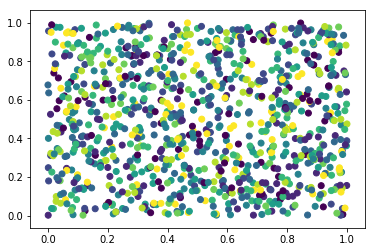
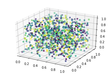
실제 데이터에서는 첫번째 인자와 두번째 인자사이의 상관관계가 있다면 그래프에서 패턴을 보실 수 있습니다. 우리는 임의의 값으로 데이터셋을 만들었으므로 예상대로 패턴을 찾을 수 없습니다. 이번에는 첫번째, 두번째, 세번째의 인자값을 이용하여 3차원으로 그래프를 확인해보겠습니다.
# 데이터셋 확인 (3차원)
from mpl_toolkits.mplot3d import Axes3D

fig = plt.figure()
ax = fig.add_subplot(111, projection='3d')

plot_x = x_train[:,0]
plot_y = x_train[:,1]
plot_z = x_train[:,2]
plot_color = y_train.reshape(1000,)

ax.scatter(plot_x, plot_y, plot_z, c=plot_color)
plt.show()
이진분류인 경우, 학습 시에는 0과 1로 값이 지정되며, 예측 시에는 0.0과 1.0 사이의 실수로 확률값이 출력됩니다. 하지만 다중클래스분류인 경우에는 클래스별로 확률값을 지정하기 위해서는 “one-hot 인코딩”을 사용합니다.
one-hot 인코딩이란 클래스가 3개일 때, 3개의 값을 가지는 행벡터로 구성하는 것을 얘기합니다. 삼각형, 사각형, 원을 구분한다고 했을 때, 학습 시에 삼각형 라벨은 [1 0 0], 사각형 라벨은 [0 1 0], 원은 [0 0 1]로 지정합니다. 출력 또한 3개의 값을 가지는 행벡터로 나오는데, 만약 [0.2 0.1 0.7] 이렇게 나왔다면, 삼각형일 확률이 20%, 사각형일 확률이 10%, 원일 확률이 70%임을 뜻하고 이를 모두 더하면 100%가 됩니다.
one-hot 인코딩은 아래 코드와 같이 케라스에서 제공하는 “to_categorical()”로 쉽게 처리할 수 있습니다
y_train = np.random.randint(10, size=(1000, 1))
y_train = to_categorical(y_train, num_classes=10) # one-hot 인코딩

y_test = np.random.randint(10, size=(100, 1))
y_test = to_categorical(y_test, num_classes=10) # one-hot 인코딩
레이어 준비
본 장에서 새롭게 소개되는 블록은 ‘softmax’입니다.
| 블록 | 이름 | 설명 |
|---|---|---|
 |
softmax | 활성화 함수로 입력되는 값을 클래스별로 확률 값이 나오도록 출력시킵니다. 이 확률값을 모두 더하면 1이 됩니다. 다중클래스 모델의 출력층에 주로 사용되며, 확률값이 가장 높은 클래스가 모델이 분류한 클래스입니다. |
모델 준비
다중클래스 분류를 하기 위해 퍼셉트론 모델, 다층퍼셉트론 모델, 깊은 다층퍼셉트론 모델을 준비했습니다.
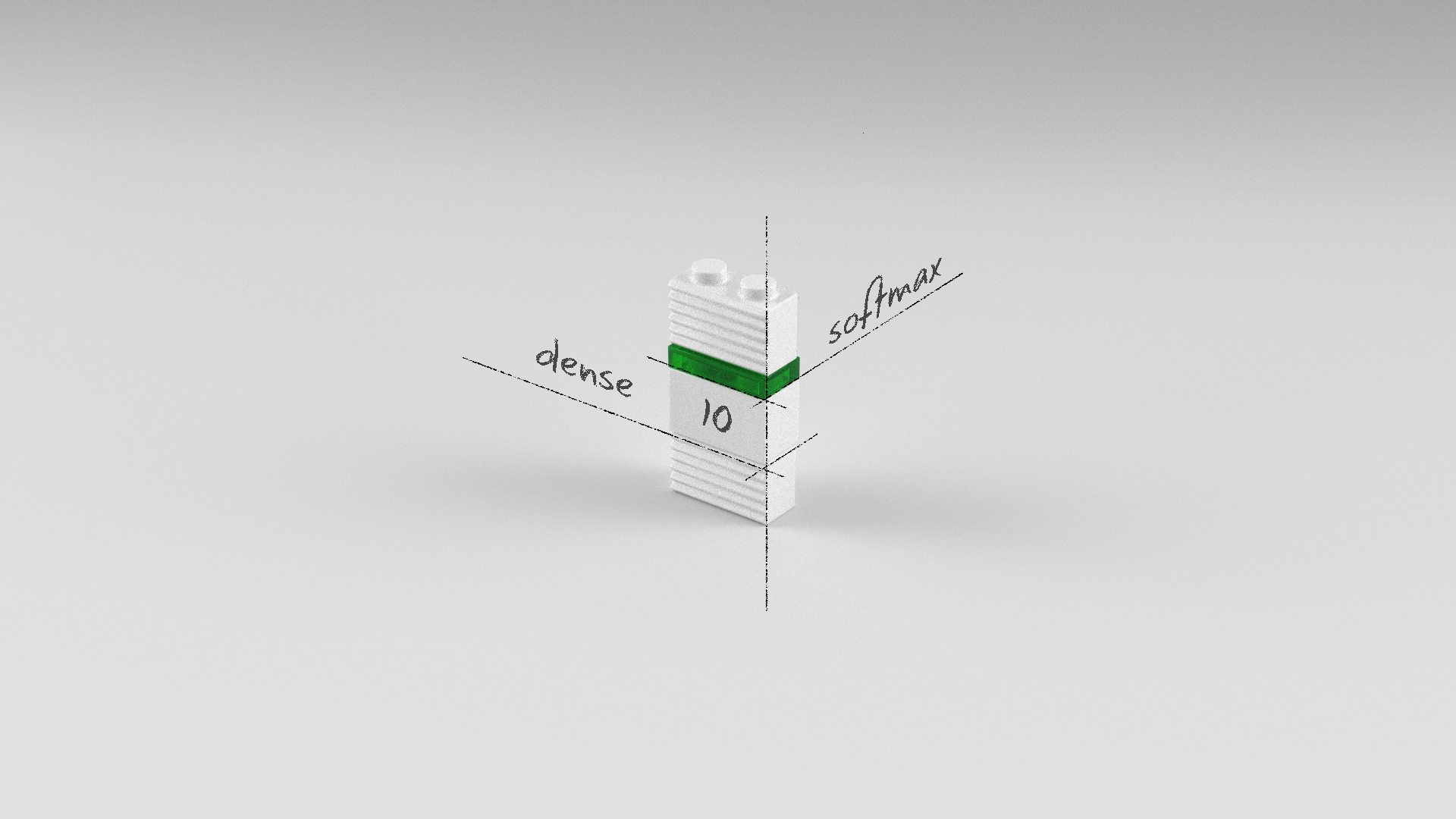
퍼셉트론 신경망 모델
Dense 레이어가 하나이고, 뉴런의 수도 하나인 가장 기본적인 퍼셉트론 모델입니다. 즉 웨이트(w) 하나, 바이어스(b) 하나로 전형적인 Y = w * X + b를 풀기 위한 모델입니다. 다중클래스분류이므로 출력 레이어는 softmax 활성화 함수를 사용하였습니다.
model = Sequential()
model.add(Dense(10, input_dim=12, activation='softmax'))
또는 활성화 함수를 브릭을 쌓듯이 별로 레이어로 구성하여도 동일한 모델입니다.
model = Sequential()
model.add(Dense(10, input_dim=12))
model.add(Activation('softmax'))
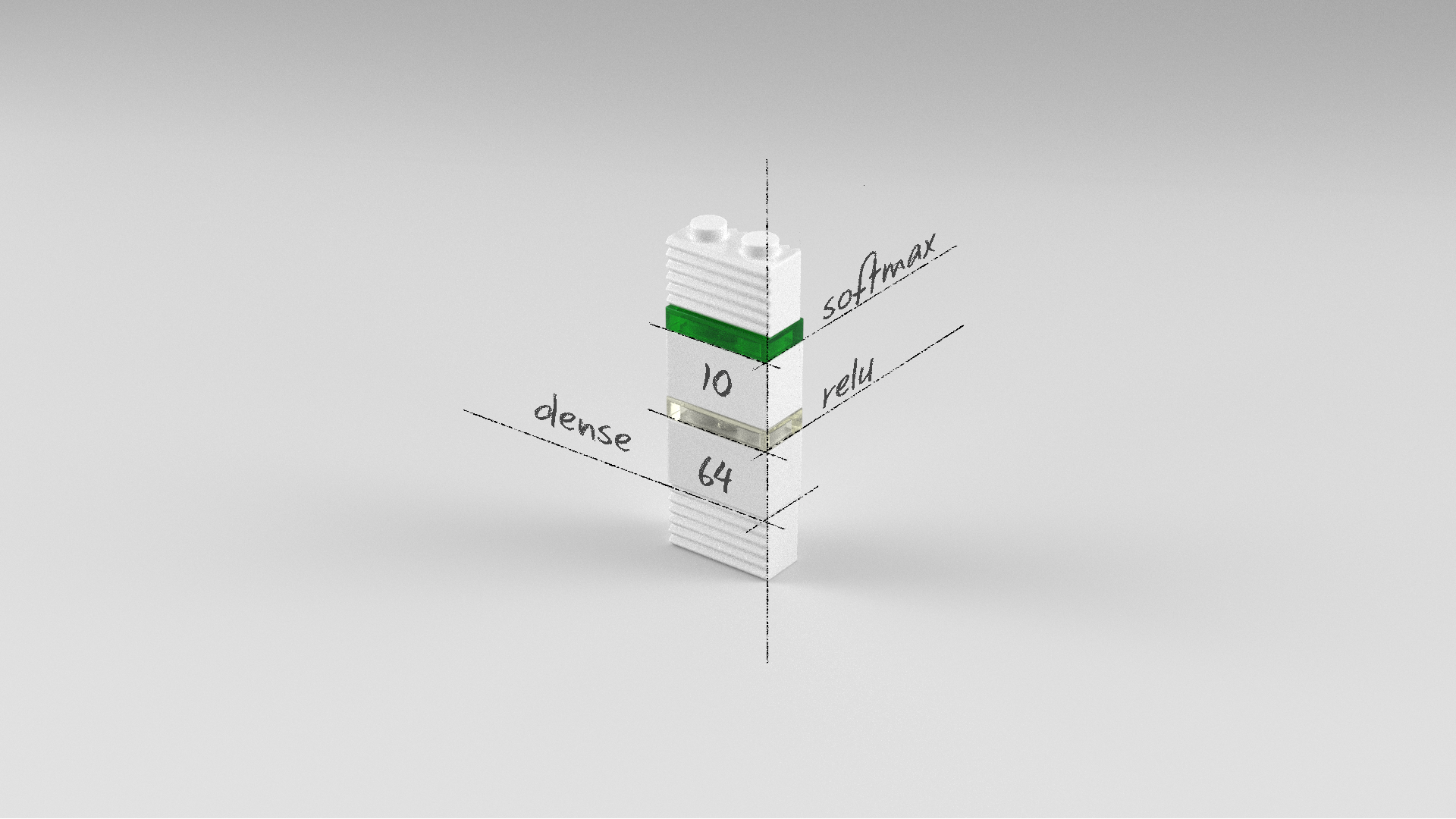
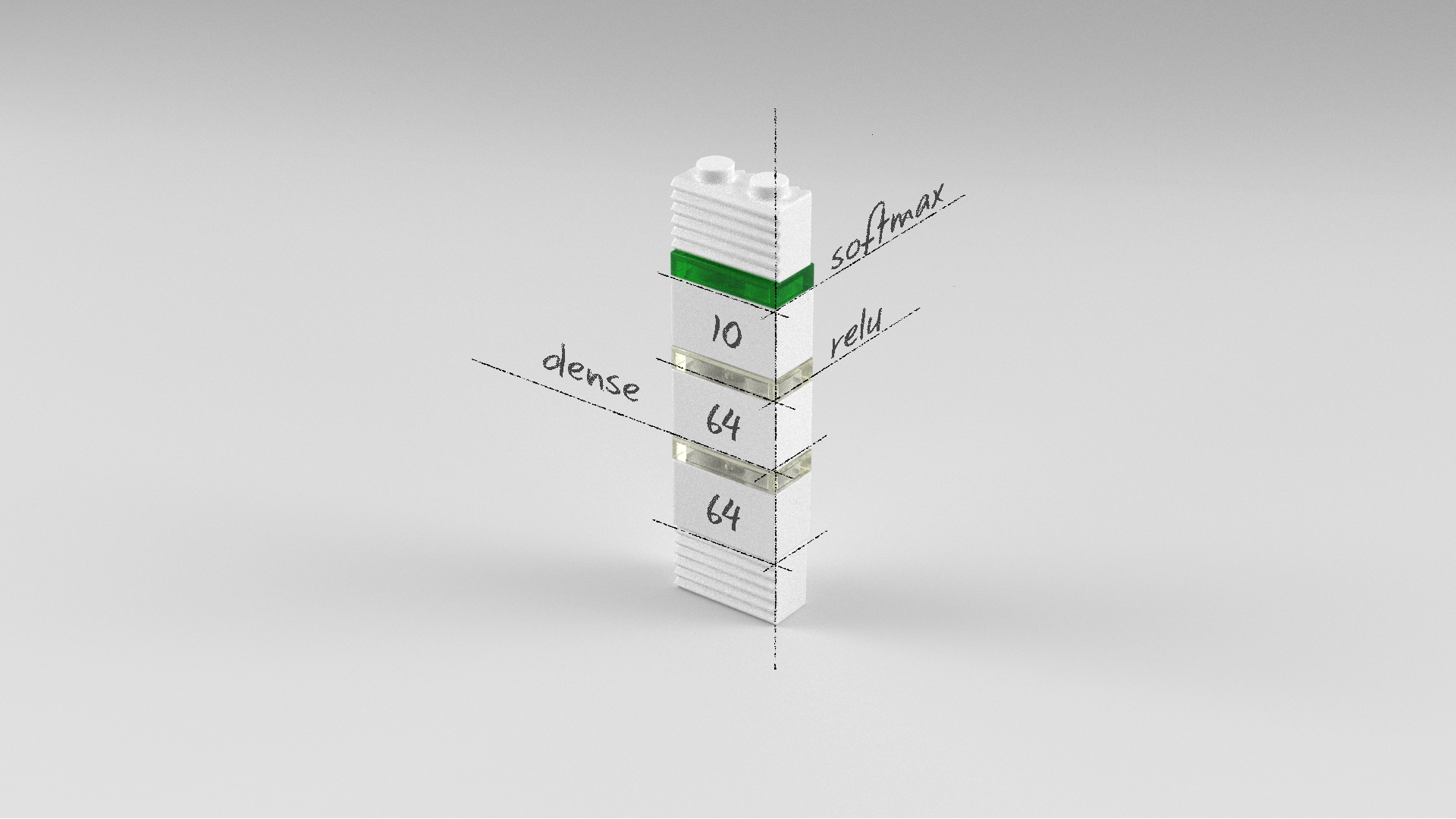
다층퍼셉트론 신경망 모델
Dense 레이어가 두 개인 다층퍼셉트론 모델입니다. 첫 번째 레이어는 64개의 뉴런을 가진 Dense 레이어이고 오류역전파가 용이한 relu 활성화 함수를 사용하였습니다. 출력 레이어인 두 번째 레이어는 클래스별 확률값을 출력하기 위해 10개의 뉴런과 softmax 활성화 함수를 사용했습니다.
model = Sequential()
model.add(Dense(64, input_dim=12, activation='relu'))
model.add(Dense(10, activation='softmax'))
깊은 다층퍼셉트론 신경망 모델
Dense 레이어가 총 세 개인 다층퍼셉트론 모델입니다. 첫 번째, 두 번째 레이어는 64개의 뉴런을 가진 Dense 레이어이고 오류역전파가 용이한 relu 활성화 함수를 사용하였습니다. 출력 레이어인 세 번째 레이어는 클래스별 확률값을 출력하기 위해 10개의 뉴런과 softmax 활성화 함수를 사용했습니다.
model = Sequential()
model.add(Dense(64, input_dim=12, activation='relu'))
model.add(Dense(64, activation='relu'))
model.add(Dense(10, activation='softmax'))
전체 소스
앞서 살펴본 퍼셉트론 신경망 모델, 다층퍼셉트론 신경망 모델, 깊은 다층퍼셉트론 신경망 모델의 전체 소스는 다음과 같습니다.
퍼셉트론 신경망 모델
# 0. 사용할 패키지 불러오기
import numpy as np
from keras.models import Sequential
from keras.layers import Dense
from keras.utils import to_categorical
import random

# 1. 데이터셋 생성하기
x_train = np.random.random((1000, 12))
y_train = np.random.randint(10, size=(1000, 1))
y_train = to_categorical(y_train, num_classes=10) # one-hot 인코딩
x_test = np.random.random((100, 12))
y_test = np.random.randint(10, size=(100, 1))
y_test = to_categorical(y_test, num_classes=10) # one-hot 인코딩

# 2. 모델 구성하기
model = Sequential()
model.add(Dense(10, input_dim=12, activation='softmax'))

# 3. 모델 학습과정 설정하기
model.compile(optimizer='rmsprop', loss='categorical_crossentropy', metrics=['accuracy'])

# 4. 모델 학습시키기
hist = model.fit(x_train, y_train, epochs=1000, batch_size=64)

# 5. 학습과정 살펴보기
%matplotlib inline
import matplotlib.pyplot as plt

fig, loss_ax = plt.subplots()

acc_ax = loss_ax.twinx()

loss_ax.set_ylim([0.0, 3.0])
acc_ax.set_ylim([0.0, 1.0])

loss_ax.plot(hist.history['loss'], 'y', label='train loss')
acc_ax.plot(hist.history['acc'], 'b', label='train acc')

loss_ax.set_xlabel('epoch')
loss_ax.set_ylabel('loss')
acc_ax.set_ylabel('accuray')

loss_ax.legend(loc='upper left')
acc_ax.legend(loc='lower left')

plt.show()

# 6. 모델 평가하기
loss_and_metrics = model.evaluate(x_test, y_test, batch_size=32)
print('loss_and_metrics : ' + str(loss_and_metrics))
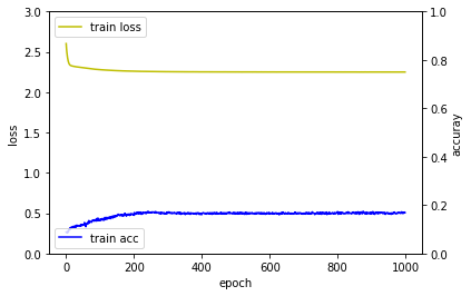
Epoch 1/1000
1000/1000 [==============================] - 0s - loss: 2.6020 - acc: 0.0880
Epoch 2/1000
1000/1000 [==============================] - 0s - loss: 2.5401 - acc: 0.0870
Epoch 3/1000
1000/1000 [==============================] - 0s - loss: 2.4952 - acc: 0.0880
...
Epoch 998/1000
1000/1000 [==============================] - 0s - loss: 2.2497 - acc: 0.1680
Epoch 999/1000
1000/1000 [==============================] - 0s - loss: 2.2495 - acc: 0.1710
Epoch 1000/1000
1000/1000 [==============================] - 0s - loss: 2.2498 - acc: 0.1690
 32/100 [========>.....................] - ETA: 0sloss_and_metrics : [2.4103073501586914, 0.089999999999999997]
다층퍼셉트론 신경망 모델
# 0. 사용할 패키지 불러오기
import numpy as np
from keras.models import Sequential
from keras.layers import Dense
from keras.utils import to_categorical
import random

# 1. 데이터셋 준비하기
x_train = np.random.random((1000, 12))
y_train = np.random.randint(10, size=(1000, 1))
y_train = to_categorical(y_train, num_classes=10) # one-hot 인코딩
x_test = np.random.random((100, 12))
y_test = np.random.randint(10, size=(100, 1))
y_test = to_categorical(y_test, num_classes=10) # one-hot 인코딩

# 2. 모델 구성하기
model = Sequential()
model.add(Dense(64, input_dim=12, activation='relu'))
model.add(Dense(10, activation='softmax'))

# 3. 모델 학습과정 설정하기
model.compile(optimizer='rmsprop', loss='categorical_crossentropy', metrics=['accuracy'])

# 4. 모델 학습시키기
hist = model.fit(x_train, y_train, epochs=1000, batch_size=64)

# 5. 학습과정 확인하기
%matplotlib inline
import matplotlib.pyplot as plt

fig, loss_ax = plt.subplots()

acc_ax = loss_ax.twinx()

loss_ax.set_ylim([0.0, 3.0])
acc_ax.set_ylim([0.0, 1.0])

loss_ax.plot(hist.history['loss'], 'y', label='train loss')
acc_ax.plot(hist.history['acc'], 'b', label='train acc')

loss_ax.set_xlabel('epoch')
loss_ax.set_ylabel('loss')
acc_ax.set_ylabel('accuray')

loss_ax.legend(loc='upper left')
acc_ax.legend(loc='lower left')

plt.show()

# 6. 모델 평가하기
loss_and_metrics = model.evaluate(x_test, y_test, batch_size=32)
print('loss_and_metrics : ' + str(loss_and_metrics))
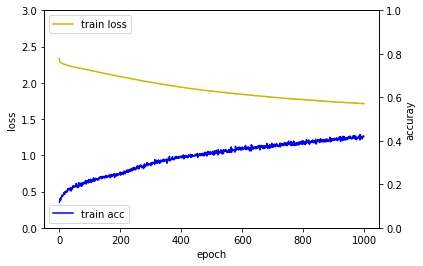
Epoch 1/1000
1000/1000 [==============================] - 0s - loss: 2.6020 - acc: 0.0880
Epoch 2/1000
1000/1000 [==============================] - 0s - loss: 2.5401 - acc: 0.0870
Epoch 3/1000
1000/1000 [==============================] - 0s - loss: 2.4952 - acc: 0.0880
...
Epoch 998/1000
1000/1000 [==============================] - 0s - loss: 1.7137 - acc: 0.4210
Epoch 999/1000
1000/1000 [==============================] - 0s - loss: 1.7149 - acc: 0.4230
Epoch 1000/1000
1000/1000 [==============================] - 0s - loss: 1.7134 - acc: 0.4190
 32/100 [========>.....................] - ETA: 0sloss_and_metrics : [2.9776978111267089, 0.12]
깊은 다층퍼셉트론 신경망 모델
# 0. 사용할 패키지 불러오기
import numpy as np
from keras.models import Sequential
from keras.layers import Dense
from keras.utils import to_categorical
import random

# 1. 데이터셋 준비하기
x_train = np.random.random((1000, 12))
y_train = np.random.randint(10, size=(1000, 1))
y_train = to_categorical(y_train, num_classes=10) # one-hot 인코딩
x_test = np.random.random((100, 12))
y_test = np.random.randint(10, size=(100, 1))
y_test = to_categorical(y_test, num_classes=10) # one-hot 인코딩

# 2. 모델 구성하기
model = Sequential()
model.add(Dense(64, input_dim=12, activation='relu'))
model.add(Dense(64, activation='relu'))
model.add(Dense(10, activation='softmax'))

# 3. 모델 학습과정 설정하기
model.compile(optimizer='rmsprop', loss='categorical_crossentropy', metrics=['accuracy'])

# 4. 모델 학습시키기
hist = model.fit(x_train, y_train, epochs=1000, batch_size=64)

# 5. 학습과정 살펴보기
%matplotlib inline
import matplotlib.pyplot as plt

fig, loss_ax = plt.subplots()

acc_ax = loss_ax.twinx()

loss_ax.set_ylim([0.0, 3.0])
acc_ax.set_ylim([0.0, 1.0])

loss_ax.plot(hist.history['loss'], 'y', label='train loss')
acc_ax.plot(hist.history['acc'], 'b', label='train acc')

loss_ax.set_xlabel('epoch')
loss_ax.set_ylabel('loss')
acc_ax.set_ylabel('accuray')

loss_ax.legend(loc='upper left')
acc_ax.legend(loc='lower left')

plt.show()

# 6. 모델 평가하기
loss_and_metrics = model.evaluate(x_test, y_test, batch_size=32)
print('loss_and_metrics : ' + str(loss_and_metrics))
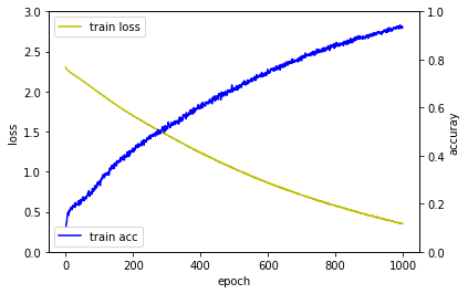
Epoch 1/1000
1000/1000 [==============================] - 0s - loss: 2.6020 - acc: 0.0880
Epoch 2/1000
1000/1000 [==============================] - 0s - loss: 2.5401 - acc: 0.0870
Epoch 3/1000
1000/1000 [==============================] - 0s - loss: 2.4952 - acc: 0.0880
...
Epoch 998/1000
1000/1000 [==============================] - 0s - loss: 0.3457 - acc: 0.9390
Epoch 999/1000
1000/1000 [==============================] - 0s - loss: 0.3538 - acc: 0.9310
Epoch 1000/1000
1000/1000 [==============================] - 0s - loss: 0.3548 - acc: 0.9340
 32/100 [========>.....................] - ETA: 0sloss_and_metrics : [5.8368307685852052, 0.089999999999999997]
학습결과 비교
퍼셉트론 신경망 모델 > 다층퍼셉트론 신경망 모델 > 깊은 다층퍼셉트론 신경망 모델 순으로 학습이 좀 더 빨리 되는 것을 확인할 수 있습니다.
| 퍼셉트론 신경망 모델 | 다층퍼셉트론 신경망 모델 | 깊은 다층퍼셉트론 신경망 모델 |
|---|---|---|
 |
 |
 |
요약
수치를 입력하여 다중클래스 분류를 할 수 있는 퍼셉트론 신경망 모델, 다층퍼셉트론 신경망 모델, 깊은 다층퍼셉트론 신경망 모델을 살펴보고, 그 성능을 확인 해봤습니다.

같이 보기
- 강좌 목차
- 이전 : 수치입력 이진분류 모델 레시피
- 다음 : 영상입력 수치예측 모델 레시피
책 소개
[추천사]
- 하용호님, 카카오 데이터사이언티스트 - 뜬구름같은 딥러닝 이론을 블록이라는 손에 잡히는 실체로 만져가며 알 수 있게 하고, 구현의 어려움은 케라스라는 시를 읽듯이 읽어내려 갈 수 있는 라이브러리로 풀어준다.
- 이부일님, (주)인사아트마이닝 대표 - 여행에서도 좋은 가이드가 있으면 여행지에 대한 깊은 이해로 여행이 풍성해지듯이 이 책은 딥러닝이라는 분야를 여행할 사람들에 가장 훌륭한 가이드가 되리라고 자부할 수 있다. 이 책을 통하여 딥러닝에 대해 보지 못했던 것들이 보이고, 듣지 못했던 것들이 들리고, 말하지 못했던 것들이 말해지는 경험을 하게 될 것이다.
- 이활석님, 네이버 클로바팀 - 레고 블럭에 비유하여 누구나 이해할 수 있게 쉽게 설명해 놓은 이 책은 딥러닝의 입문 도서로서 제 역할을 다 하리라 믿습니다.
- 김진중님, 야놀자 Head of STL - 복잡했던 머릿속이 맑고 깨끗해지는 효과가 있습니다.
- 이태영님, 신한은행 디지털 전략부 AI LAB - 기존의 텐서플로우를 활용했던 분들에게 바라볼 수 있는 관점의 전환점을 줄 수 있는 Mild Stone과 같은 책이다.
- 전태균님, 쎄트렉아이 - 케라스의 특징인 단순함, 확장성, 재사용성을 눈으로 쉽게 보여주기 위해 친절하게 정리된 내용이라 생각합니다.
- 유재준님, 카이스트 - 바로 적용해보고 싶지만 어디부터 시작할지 모를 때 최선의 선택입니다.