클래스별로 학습과정 살펴보기

fit() 함수 로그에는 기본적으로 손실값과 정확도가 표시됩니다. 이진분류 모델에서는 정확도값 하나만 보더라도 학습이 제대로 되고 있는 지 알 수 있지만, 다중클래스분류 문제에서는 클래스별로 학습이 제대로 되고 있는 지 확인하기 위해서는 정확도값 하나로는 부족함이 많습니다. 이진분류 문제에서 클래스간 불균형이 있을 경우에도 정확도값 하나로는 판단할 수가 없습니다. 본 장에서는 학습 중에 클래스별로 정밀도(precision)와 재현율(recall)을 살펴볼 수 있도록 사용자 정의 메트릭(custom metric)을 사용하는 법과 나온 결과를 시각화 하는 방법을 알아보겠습니다.

메트릭 개념

메트릭은 평가 기준을 말합니다. compile() 함수의 metrics 인자로 여러 개의 평가 기준을 지정할 수 있습니다. 이러한 평가 기준에는 모델의 학습에는 영향을 미치지 않지만, 학습 과정 중에 제대로 학습되고 있는 지 살펴볼 수 있습니다. 아래는 일반적으로 평가 기준을 ‘accuracy’으로 삽입하였을 때의 코드입니다.

model.compile(loss='categorical_crossentropy', optimizer='sgd', metrics=['accuracy'])

케라스에서는 다중클래스분류 문제에서 평가기준을 ‘accuracy’로 지정했을 경우 내부적으로 categorical_accuracy() 함수를 이용하여 정확도가 계산됩니다.

def categorical_accuracy(y_true, y_pred):
    return K.cast(K.equal(K.argmax(y_true, axis=-1),
                          K.argmax(y_pred, axis=-1)),
                  K.floatx())

이런 평가 기준을 정의하는 함수는 두 개의 인자를 받습니다.

y_true: 실제 값, 티아노 및 텐스플로우의 텐서(tensor)
y_pred: 예측 값, 티아노 및 텐스플로우의 텐서(tensor)

함수 내부는 어떻게 평가를 할 것인가를 정의합니다. 이 함수는 매 배치때마다 호출되며 입력되는 데이터들에 대해 평가를 수행한 후 그 결과의 평균을 하나의 텐서로 반환합니다.

사용자 정의 메트릭

케라스에서 제공하는 함수형태와 비슷하게 사용자 정의 메트릭을 만들 수 있습니다. 아래 코드는 특정 클래스에 대한 정밀도를 평가하는 함수입니다. 여러 개의 클래스를 하나의 함수로 사용할 수 있도록 ‘interesting_class_id’ 인자를 사용하였습니다.

def single_class_precision(interesting_class_id):
    def prec(y_true, y_pred):
        class_id_true = K.argmax(y_true, axis=-1)
        class_id_pred = K.argmax(y_pred, axis=-1)
        precision_mask = K.cast(K.equal(class_id_pred, interesting_class_id), 'int32')
        class_prec_tensor = K.cast(K.equal(class_id_true, class_id_pred), 'int32') * precision_mask
        class_prec = K.cast(K.sum(class_prec_tensor), 'float32') / K.cast(K.maximum(K.sum(precision_mask), 1), 'float32')
        return class_prec
    return prec

분류 문제에서 클래스별로 확인할 때는 정밀도와 재현율을 파악하는 것이 도움이 됩니다. 정밀도와 재현율의 개념에 대해서는 ‘평가 이야기’을 참고하시기 바랍니다. 아래 코드는 특정 클래스에 대한 재현율을 평가하는 함수입니다.

def single_class_recall(interesting_class_id):
    def recall(y_true, y_pred):
        class_id_true = K.argmax(y_true, axis=-1)
        class_id_pred = K.argmax(y_pred, axis=-1)
        recall_mask = K.cast(K.equal(class_id_true, interesting_class_id), 'int32')
        class_recall_tensor = K.cast(K.equal(class_id_true, class_id_pred), 'int32') * recall_mask
        class_recall = K.cast(K.sum(class_recall_tensor), 'float32') / K.cast(K.maximum(K.sum(recall_mask), 1), 'float32')
        return class_recall
    return recall

사용자 정의 메트릭 사용하기

사용자 정의 메트릭을 사용할 때는 compile() 함수의 metrics 인자에 함수명을 삽입합니다. ‘interesting_class_id’ 인자를 사용하였으므로, 클래스 인덱스를 넘기도록 합니다. 본 예제에서는 mnist을 사용하기 때문에 0~9까지로 살펴보도록 하겠습니다.

model.compile(loss='categorical_crossentropy', optimizer='sgd', 
              metrics=['accuracy',
                       single_class_precision(0), single_class_recall(0),
                       single_class_precision(1), single_class_recall(1),
                       single_class_precision(2), single_class_recall(2),
                       single_class_precision(3), single_class_recall(3),
                       single_class_precision(4), single_class_recall(4),
                       single_class_precision(5), single_class_recall(5),
                       single_class_precision(6), single_class_recall(6),
                       single_class_precision(7), single_class_recall(7),
                       single_class_precision(8), single_class_recall(8),
                       single_class_precision(9), single_class_recall(9)])

학습과정 살펴보기

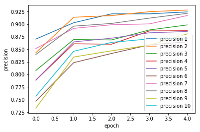
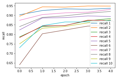
fit() 함수는 히스토리 객체를 반환하는 데, 이 객체에는 매 에포크마다 prec_1, prec_2, prec_3… prec_10과 recall_1, recall_2, recall_3… recall_10의 값을 가지고 있습니다.

hist = model.fit(x_train, y_train, epochs=5, batch_size=32)

메트릭을 여러개 지정할 경우 아래와 같이 fit() 함수 실행 시 로그에도 여러 개의 메트릭이 표시됩니다. 동시에 여러 수치가 올라가는 것을 보고있노라면 마치 참새가 재잘거리는 소리가 들리는 것 같군요.

이 값을 시각화하는 코드는 다음과 같습니다.

%matplotlib inline
import matplotlib.pyplot as plt

plt.plot(hist.history['prec_1'], label='precision 1')
plt.plot(hist.history['prec_2'], label='precision 2')
plt.plot(hist.history['prec_3'], label='precision 3')
plt.plot(hist.history['prec_4'], label='precision 4')
plt.plot(hist.history['prec_5'], label='precision 5')
plt.plot(hist.history['prec_6'], label='precision 6')
plt.plot(hist.history['prec_7'], label='precision 7')
plt.plot(hist.history['prec_8'], label='precision 8')
plt.plot(hist.history['prec_9'], label='precision 9')
plt.plot(hist.history['prec_10'], label='precision 10')
plt.xlabel('epoch')
plt.ylabel('precision')
plt.legend(loc='lower right')
plt.show()

plt.plot(hist.history['recall_1'], label='recall 1')
plt.plot(hist.history['recall_2'], label='recall 2')
plt.plot(hist.history['recall_3'], label='recall 3')
plt.plot(hist.history['recall_4'], label='recall 4')
plt.plot(hist.history['recall_5'], label='recall 5')
plt.plot(hist.history['recall_6'], label='recall 6')
plt.plot(hist.history['recall_7'], label='recall 7')
plt.plot(hist.history['recall_8'], label='recall 8')
plt.plot(hist.history['recall_9'], label='recall 9')
plt.plot(hist.history['recall_10'], label='recall 10')
plt.xlabel('epoch')
plt.ylabel('recall')
plt.legend(loc='lower right')
plt.show()

메트릭을 이용한 평가결과 살펴보기

evaluate() 함수는 손실값 및 메트릭 값을 반환하는 데, 여러 메트릭을 정의 및 등록하였으므로, 여러 개의 메트릭 값을 얻을 수 있습니다.

loss_and_metrics = model.evaluate(x_test, y_test, batch_size=32)

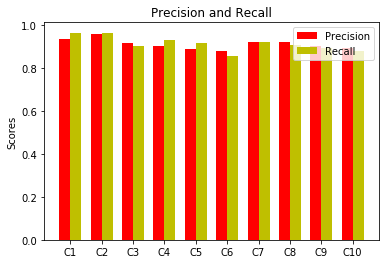
아래는 평가를 통해 얻은 메트릭 값을 시각화하는 코드입니다. 클래스별로 정밀도와 재현율을 막대그래프로 표시해봤습니다.

import numpy as np

metrics = np.array(loss_and_metrics[2:])
idx = np.linspace(0, 19, 20) 
precision = metrics[(idx % 2) == 0]
recall = metrics[((idx+1) % 2) == 0]

import matplotlib.pyplot as plt

N = 10
ind = np.arange(N)
width = 0.35

fig, ax = plt.subplots()
prec_bar = ax.bar(ind, precision, width, color='r')
recall_bar = ax.bar(ind + width, recall, width, color='y')

ax.set_ylabel('Scores')
ax.set_title('Precision and Recall')
ax.set_xticks(ind + width / 2)
ax.set_xticklabels(('C1', 'C2', 'C3', 'C4', 'C5', 'C6', 'C7', 'C8', 'C9', 'C10'))

ax.legend((prec_bar[0], recall_bar[0]), ('Precision', 'Recall'))

plt.show()

전체 소스코드

전체 소스코드는 다음과 같습니다. 기본적인 mnist 예제에서 사용자 정의 메트릭 정의 및 등록과 시각화 하는 부분이 추가되었습니다.

# 0. 사용할 패키지 불러오기
from keras.utils import np_utils
from keras.datasets import mnist
from keras.models import Sequential
from keras.layers import Dense, Activation

from keras import backend as K

# 특정 클래스에 대한 정밀도
def single_class_precision(interesting_class_id):
    def prec(y_true, y_pred):
        class_id_true = K.argmax(y_true, axis=-1)
        class_id_pred = K.argmax(y_pred, axis=-1)
        precision_mask = K.cast(K.equal(class_id_pred, interesting_class_id), 'int32')
        class_prec_tensor = K.cast(K.equal(class_id_true, class_id_pred), 'int32') * precision_mask
        class_prec = K.cast(K.sum(class_prec_tensor), 'float32') / K.cast(K.maximum(K.sum(precision_mask), 1), 'float32')
        return class_prec
    return prec

# 특정 클래스에 대한 재현율
def single_class_recall(interesting_class_id):
    def recall(y_true, y_pred):
        class_id_true = K.argmax(y_true, axis=-1)
        class_id_pred = K.argmax(y_pred, axis=-1)
        recall_mask = K.cast(K.equal(class_id_true, interesting_class_id), 'int32')
        class_recall_tensor = K.cast(K.equal(class_id_true, class_id_pred), 'int32') * recall_mask
        class_recall = K.cast(K.sum(class_recall_tensor), 'float32') / K.cast(K.maximum(K.sum(recall_mask), 1), 'float32')
        return class_recall
    return recall

# 1. 데이터셋 생성하기
(x_train, y_train), (x_test, y_test) = mnist.load_data()
x_train = x_train.reshape(60000, 784).astype('float32') / 255.0
x_test = x_test.reshape(10000, 784).astype('float32') / 255.0
y_train = np_utils.to_categorical(y_train)
y_test = np_utils.to_categorical(y_test)

# 2. 모델 구성하기
model = Sequential()
model.add(Dense(units=64, input_dim=28*28, activation='relu'))
model.add(Dense(units=10, activation='softmax'))

# 3. 모델 학습과정 설정하기
model.compile(loss='categorical_crossentropy', optimizer='sgd', 
              metrics=['accuracy',
                       single_class_precision(0), single_class_recall(0),
                       single_class_precision(1), single_class_recall(1),
                       single_class_precision(2), single_class_recall(2),
                       single_class_precision(3), single_class_recall(3),
                       single_class_precision(4), single_class_recall(4),
                       single_class_precision(5), single_class_recall(5),
                       single_class_precision(6), single_class_recall(6),
                       single_class_precision(7), single_class_recall(7),
                       single_class_precision(8), single_class_recall(8),
                       single_class_precision(9), single_class_recall(9)])

# 4. 모델 학습시키기
hist = model.fit(x_train, y_train, epochs=5, batch_size=32)

# 5. 학습과정 살펴보기
%matplotlib inline
import matplotlib.pyplot as plt

plt.plot(hist.history['prec_1'], label='precision 1')
plt.plot(hist.history['prec_2'], label='precision 2')
plt.plot(hist.history['prec_3'], label='precision 3')
plt.plot(hist.history['prec_4'], label='precision 4')
plt.plot(hist.history['prec_5'], label='precision 5')
plt.plot(hist.history['prec_6'], label='precision 6')
plt.plot(hist.history['prec_7'], label='precision 7')
plt.plot(hist.history['prec_8'], label='precision 8')
plt.plot(hist.history['prec_9'], label='precision 9')
plt.plot(hist.history['prec_10'], label='precision 10')
plt.xlabel('epoch')
plt.ylabel('precision')
plt.legend(loc='lower right')
plt.show()

plt.plot(hist.history['recall_1'], label='recall 1')
plt.plot(hist.history['recall_2'], label='recall 2')
plt.plot(hist.history['recall_3'], label='recall 3')
plt.plot(hist.history['recall_4'], label='recall 4')
plt.plot(hist.history['recall_5'], label='recall 5')
plt.plot(hist.history['recall_6'], label='recall 6')
plt.plot(hist.history['recall_7'], label='recall 7')
plt.plot(hist.history['recall_8'], label='recall 8')
plt.plot(hist.history['recall_9'], label='recall 9')
plt.plot(hist.history['recall_10'], label='recall 10')
plt.xlabel('epoch')
plt.ylabel('recall')
plt.legend(loc='lower right')
plt.show()

# 6. 모델 평가하기
loss_and_metrics = model.evaluate(x_test, y_test, batch_size=32)
print('## evaluation loss and_metrics ##')
print(loss_and_metrics)

import numpy as np

metrics = np.array(loss_and_metrics[2:])
idx = np.linspace(0, 19, 20) 
precision = metrics[(idx % 2) == 0]
recall = metrics[((idx+1) % 2) == 0]

import matplotlib.pyplot as plt

N = 10
ind = np.arange(N)
width = 0.35

fig, ax = plt.subplots()
prec_bar = ax.bar(ind, precision, width, color='r')
recall_bar = ax.bar(ind + width, recall, width, color='y')

ax.set_ylabel('Scores')
ax.set_title('Precision and Recall')
ax.set_xticks(ind + width / 2)
ax.set_xticklabels(('C1', 'C2', 'C3', 'C4', 'C5', 'C6', 'C7', 'C8', 'C9', 'C10'))

ax.legend((prec_bar[0], recall_bar[0]), ('Precision', 'Recall'))

plt.show()

Epoch 1/5
60000/60000 [==============================] - 7s - loss: 0.6639 - acc: 0.8324 - prec_1: 0.8705 - recall_1: 0.9026 - prec_2: 0.8434 - recall_2: 0.8951 - prec_3: 0.8080 - recall_3: 0.7866 - prec_4: 0.7888 - recall_4: 0.7829 - prec_5: 0.7889 - recall_5: 0.8232 - prec_6: 0.7472 - recall_6: 0.6403 - prec_7: 0.8516 - recall_7: 0.8736 - prec_8: 0.8397 - recall_8: 0.8406 - prec_9: 0.7332 - recall_9: 0.7501 - prec_10: 0.7570 - recall_10: 0.7301     
Epoch 2/5
60000/60000 [==============================] - 7s - loss: 0.3468 - acc: 0.9031 - prec_1: 0.9029 - recall_1: 0.9249 - prec_2: 0.9138 - recall_2: 0.9442 - prec_3: 0.8696 - recall_3: 0.8409 - prec_4: 0.8610 - recall_4: 0.8441 - prec_5: 0.8648 - recall_5: 0.8857 - prec_6: 0.8236 - recall_6: 0.8028 - prec_7: 0.8917 - recall_7: 0.9036 - prec_8: 0.8961 - recall_8: 0.8888 - prec_9: 0.8348 - recall_9: 0.8321 - prec_10: 0.8462 - recall_10: 0.8455     
Epoch 3/5
60000/60000 [==============================] - 7s - loss: 0.3002 - acc: 0.9155 - prec_1: 0.9206 - recall_1: 0.9337 - prec_2: 0.9171 - recall_2: 0.9430 - prec_3: 0.8687 - recall_3: 0.8467 - prec_4: 0.8603 - recall_4: 0.8460 - prec_5: 0.8722 - recall_5: 0.8878 - prec_6: 0.8418 - recall_6: 0.8227 - prec_7: 0.8988 - recall_7: 0.9126 - prec_8: 0.9015 - recall_8: 0.8970 - prec_9: 0.8471 - recall_9: 0.8412 - prec_10: 0.8639 - recall_10: 0.8648     
Epoch 4/5
60000/60000 [==============================] - 7s - loss: 0.2718 - acc: 0.9238 - prec_1: 0.9206 - recall_1: 0.9314 - prec_2: 0.9248 - recall_2: 0.9486 - prec_3: 0.8886 - recall_3: 0.8712 - prec_4: 0.8866 - recall_4: 0.8744 - prec_5: 0.8829 - recall_5: 0.8966 - prec_6: 0.8589 - recall_6: 0.8432 - prec_7: 0.9006 - recall_7: 0.9161 - prec_8: 0.9120 - recall_8: 0.9102 - prec_9: 0.8584 - recall_9: 0.8601 - prec_10: 0.8708 - recall_10: 0.8654     
Epoch 5/5
60000/60000 [==============================] - 8s - loss: 0.2497 - acc: 0.9298 - prec_1: 0.9244 - recall_1: 0.9368 - prec_2: 0.9281 - recall_2: 0.9482 - prec_3: 0.8985 - recall_3: 0.8828 - prec_4: 0.8871 - recall_4: 0.8728 - prec_5: 0.8855 - recall_5: 0.8935 - prec_6: 0.8650 - recall_6: 0.8475 - prec_7: 0.9172 - recall_7: 0.9309 - prec_8: 0.9215 - recall_8: 0.9202 - prec_9: 0.8807 - recall_9: 0.8760 - prec_10: 0.8724 - recall_10: 0.8728     

 9664/10000 [===========================>..] - ETA: 0s## evaluation loss and_metrics ##
[0.23389623485803604, 0.93569999999999998, 0.93501714344024656, 0.96290285758972172, 0.95712000045776369, 0.95975619077682495, 0.91664761981964116, 0.90009523944854741, 0.90259047775268553, 0.92727619199752809, 0.886011429977417, 0.91370666770935061, 0.87623619136810305, 0.85451682758331304, 0.92037333421707157, 0.92180571537017819, 0.9204723814964294, 0.90364190587997439, 0.90296889028549199, 0.89279238224029545, 0.88955913543701171, 0.87660952548980708]

요약

다중클래스분류 문제에서 클래스별로 정밀도 및 재현율을 알아보기 위해 사용자 정의 메트릭을 정의하고 등록하는 법을 알아보왔습니다. 그리고 학습 과정 및 평가 시에 산출되는 메트릭 값을 차트를 통해 시각화하는 방법에 대해서도 알아봤습니다. 이 방법들을 통해 ‘accuracy’ 값만 보던 것을 벗어나 다양한 평가 기준으로 모델의 학습과정을 살펴보시기 바랍니다.