영상입력 수치예측 모델 레시피
영상을 입력해서 수치를 예측하는 모델들에 대해서 알아보겠습니다. 간단한 테스트를 위해 수치예측을 위한 영상 데이터셋 생성을 해보고, 다층퍼셉트론 및 컨볼루션 신경망 모델을 구성 및 학습 시켜보겠습니다. 이 모델은 고정된 지역에서 촬영된 영상으로부터 복잡도, 밀도 등을 수치화하는 문제를 풀 수 있습니다. 아래 문제들에 활용 기대해봅니다.
- CCTV 등 촬영 영상으로부터 미세먼지 지수 예측
- 위성영상으로부터 녹조, 적조 등의 지수 예측
- 태양광 패널의 먼지가 쌓여있는 정도 예측
데이터셋 준비
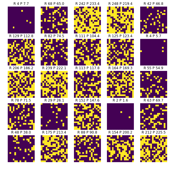
너비가 16, 높이가 16이고, 픽셀값을 0과 1을 가지는 영상을 만들어보겠습니다. 임의의 값이 주어지면, 그 값만큼 반복하여 영상 내에 1인 픽셀을 찍었습니다. 여기서 임의의 값이 라벨값으로 지정했습니다.
width = 16
height = 16

def generate_dataset(samples):

    ds_x = []
    ds_y = []

    for it in range(samples):

        num_pt = np.random.randint(0, width * height)
        img = generate_image(num_pt)

        ds_y.append(num_pt)
        ds_x.append(img)

    return np.array(ds_x), np.array(ds_y).reshape(samples, 1)

def generate_image(points):

    img = np.zeros((width, height))
    pts = np.random.random((points, 2))

    for ipt in pts:
        img[int(ipt[0] * width), int(ipt[1] * height)] = 1

    return img.reshape(width, height, 1)
데이터셋으로 훈련셋을 1500개, 검증셋을 300개, 시험셋을 100개 생성합니다.
x_train, y_train = generate_dataset(1500)
x_val, y_val = generate_dataset(300)
x_test, y_test = generate_dataset(100)
만든 데이터셋 일부를 가시화 해보겠습니다.
%matplotlib inline
import matplotlib.pyplot as plt

plt_row = 5
plt_col = 5

plt.rcParams["figure.figsize"] = (10,10)

f, axarr = plt.subplots(plt_row, plt_col)

for i in range(plt_row*plt_col):
    sub_plt = axarr[i/plt_row, i%plt_col]
    sub_plt.axis('off')
    sub_plt.imshow(x_train[i].reshape(width, height))
    sub_plt.set_title('R ' + str(y_train[i][0]))

plt.show()
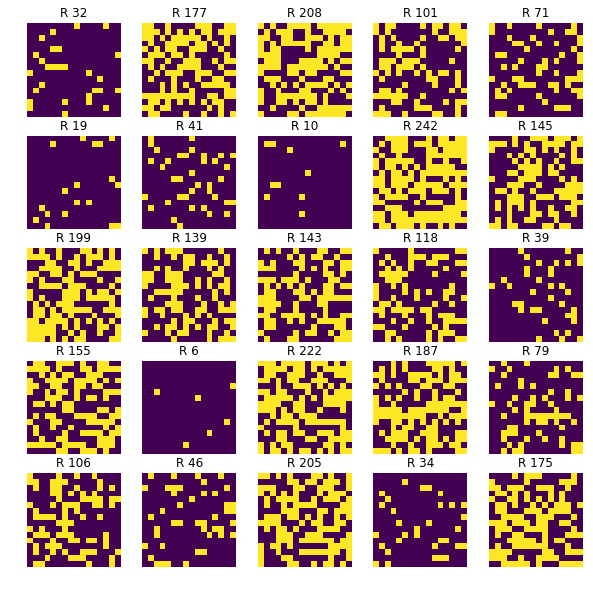
R(Real)은 1인 값을 가진 픽셀 수를 의미합니다. 한 번 표시한 픽셀에 다시 표시가 될 수 있기 때문에 실제 픽셀 수와 조금 차이는 날 수 있습니다.
레이어 준비
본 장에서 새롭게 소개되는 블록들은 다음과 같습니다.
| 블록 | 이름 | 설명 |
|---|---|---|
 |
2D Input data | 2차원의 입력 데이터입니다. 주로 영상 데이터를 의미하며, 너비, 높이, 채널수로 구성됩니다. |
 |
Conv2D | 필터를 이용하여 영상 특징을 추출하는 컨볼루션 레이어입니다. |
 |
MaxPooling2D | 영상에서 사소한 변화가 특징 추출에 크게 영향을 미치지 않도록 해주는 맥스풀링 레이어입니다. |
 |
Flatten | 2차원의 특징맵을 전결합층으로 전달하기 위해서 1차원 형식으로 바꿔줍니다. |
 |
relu | 활성화 함수로 주로 Conv2D 은닉층에 사용됩니다. |
모델 준비
영상입력 수치예측을 하기 위해 다층퍼셉트론 신경망 모델, 컨볼루션 신경망 모델을 준비했습니다.
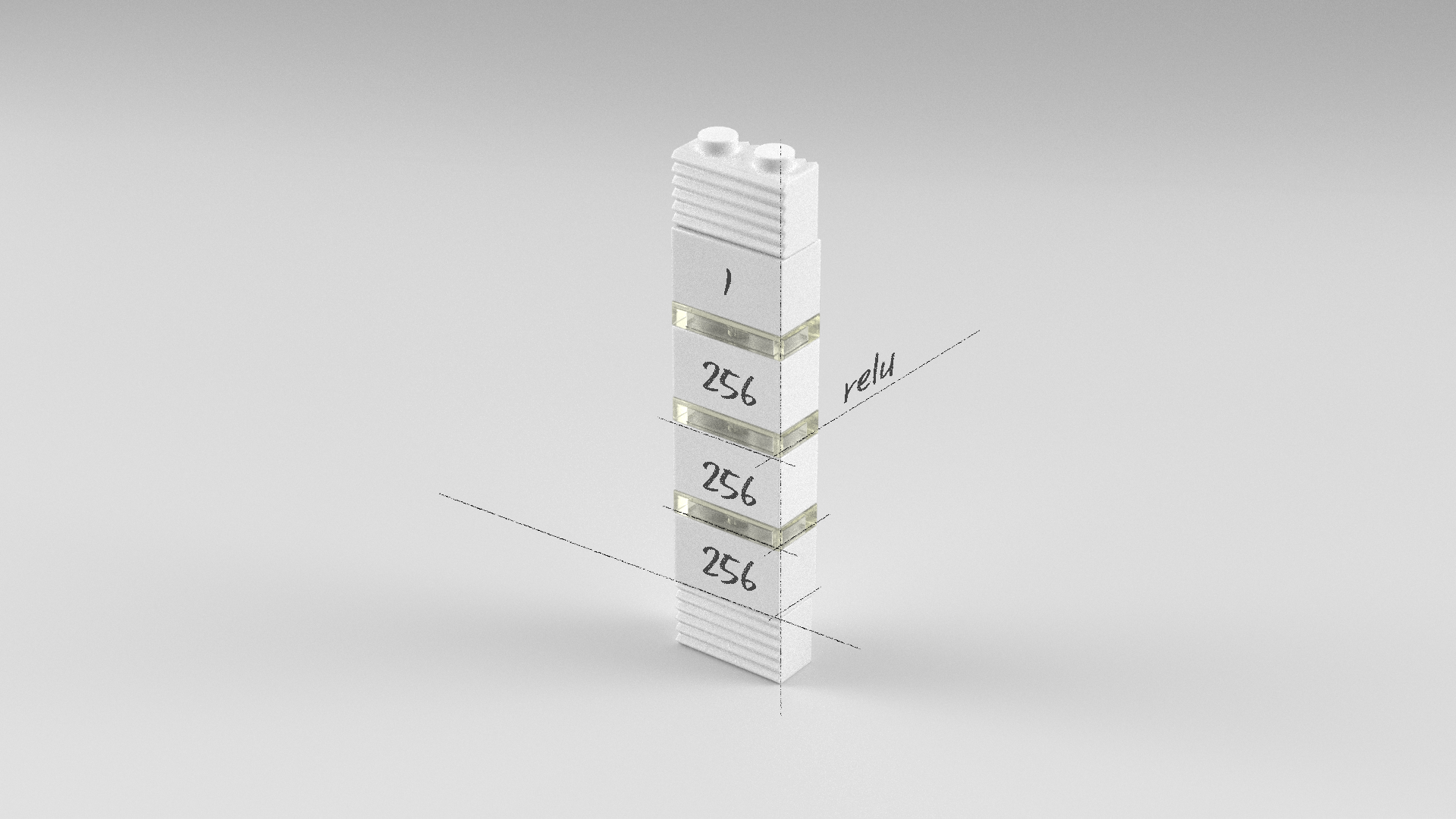
다층퍼셉트론 신경망 모델
model = Sequential()
model.add(Dense(256, activation='relu', input_dim = width*height))
model.add(Dense(256, activation='relu'))
model.add(Dense(256))
model.add(Dense(1))
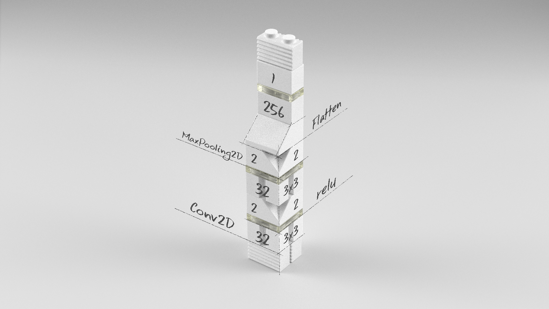
컨볼루션 신경망 모델
model = Sequential()
model.add(Conv2D(32, (3, 3), activation='relu', input_shape=(width, height, 1)))
model.add(MaxPooling2D(pool_size=(2, 2)))
model.add(Conv2D(32, (3, 3), activation='relu'))
model.add(MaxPooling2D(pool_size=(2, 2)))
model.add(Flatten())
model.add(Dense(256, activation='relu'))
model.add(Dense(1))
전체 소스
앞서 살펴본 다층퍼셉트론 신경망 모델, 컨볼루션 신경망 모델의 전체 소스는 다음과 같습니다.
다층퍼셉트론 신경망 모델
# 0. 사용할 패키지 불러오기
import numpy as np
from keras.models import Sequential
from keras.layers import Dense

width = 16
height = 16

def generate_dataset(samples):

    ds_x = []
    ds_y = []

    for it in range(samples):

        num_pt = np.random.randint(0, width * height)
        img = generate_image(num_pt)

        ds_y.append(num_pt)
        ds_x.append(img)

    return np.array(ds_x), np.array(ds_y).reshape(samples, 1)

def generate_image(points):

    img = np.zeros((width, height))
    pts = np.random.random((points, 2))

    for ipt in pts:
        img[int(ipt[0] * width), int(ipt[1] * height)] = 1

    return img.reshape(width, height, 1)

# 1. 데이터셋 생성하기
x_train, y_train = generate_dataset(1500)
x_val, y_val = generate_dataset(300)
x_test, y_test = generate_dataset(100)

x_train_1d = x_train.reshape(x_train.shape[0], width*height)
x_val_1d = x_val.reshape(x_val.shape[0], width*height)
x_test_1d = x_test.reshape(x_test.shape[0], width*height)

# 2. 모델 구성하기
model = Sequential()
model.add(Dense(256, activation='relu', input_dim = width*height))
model.add(Dense(256, activation='relu'))
model.add(Dense(256))
model.add(Dense(1))

# 3. 모델 학습과정 설정하기
model.compile(loss='mse', optimizer='adam')

# 4. 모델 학습시키기
hist = model.fit(x_train_1d, y_train, batch_size=32, epochs=1000, validation_data=(x_val_1d, y_val))

# 5. 학습과정 살펴보기
%matplotlib inline
import matplotlib.pyplot as plt

plt.plot(hist.history['loss'])
plt.plot(hist.history['val_loss'])
plt.ylim(0.0, 300.0)
plt.ylabel('loss')
plt.xlabel('epoch')
plt.legend(['train', 'val'], loc='upper left')
plt.show()

# 6. 모델 평가하기
score = model.evaluate(x_test_1d, y_test, batch_size=32)

print(score)

# 7. 모델 사용하기
yhat_test = model.predict(x_test_1d, batch_size=32)

%matplotlib inline
import matplotlib.pyplot as plt

plt_row = 5
plt_col = 5

plt.rcParams["figure.figsize"] = (10,10)

f, axarr = plt.subplots(plt_row, plt_col)

for i in range(plt_row*plt_col):
    sub_plt = axarr[i//plt_row, i%plt_col]
    sub_plt.axis('off')
    sub_plt.imshow(x_test[i].reshape(width, height))
    sub_plt.set_title('R %d P %.1f' % (y_test[i][0], yhat_test[i][0]))

plt.show()
Train on 1500 samples, validate on 300 samples
Epoch 1/1000
1500/1500 [==============================] - 0s 319us/step - loss: 4512.4429 - val_loss: 277.1421
Epoch 2/1000
1500/1500 [==============================] - 0s 74us/step - loss: 251.0093 - val_loss: 205.3613
Epoch 3/1000
1500/1500 [==============================] - 0s 74us/step - loss: 199.9910 - val_loss: 158.1126
...
Epoch 998/1000
1500/1500 [==============================] - 0s 92us/step - loss: 0.0384 - val_loss: 72.1721
Epoch 999/1000
1500/1500 [==============================] - 0s 89us/step - loss: 0.0298 - val_loss: 71.9559
Epoch 1000/1000
1500/1500 [==============================] - 0s 69us/step - loss: 0.0534 - val_loss: 71.9296

100/100 [==============================] - 0s 46us/step
61.79263580322266
다층퍼셉트론 모델의 입력층인 Dense 레이어는 일차원 벡터로 데이터를 입력 받기 때문에, 이차원인 영상을 일차원 벡터로 변환하는 과정이 필요합니다.
x_train_1d = x_train.reshape(x_train.shape[0], width*height)
x_val_1d = x_val.reshape(x_val.shape[0], width*height)
x_test_1d = x_test.reshape(x_test.shape[0], width*height)
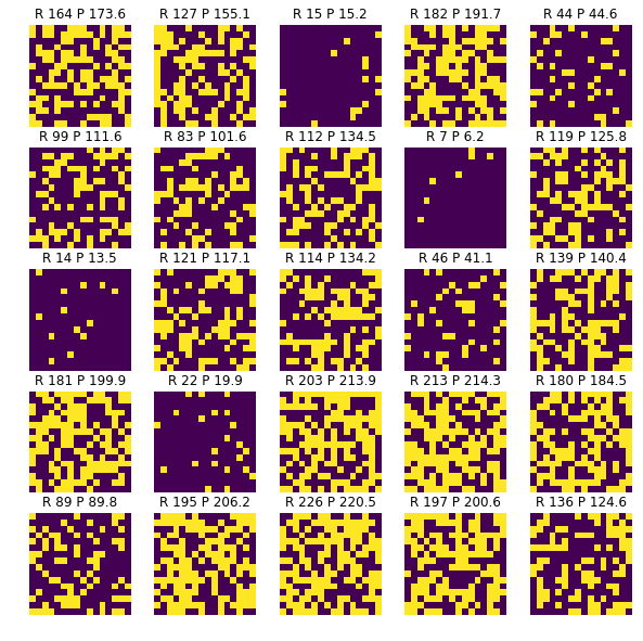
예측 결과 일부를 표시해봤습니다. R(Real)이 실제 값이고, P(Prediction)이 모델이 예측한 결과입니다. 출력층에 따로 활성화 함수를 지정하지 않았기 때문에 선형 함수가 사용되며, 정수가 아닌 실수로 예측됩니다.
컨볼루션 신경망 모델
# 0. 사용할 패키지 불러오기
import numpy as np
from keras.models import Sequential
from keras.layers import Dense, Dropout, Flatten
from keras.layers import Conv2D, MaxPooling2D

width = 16
height = 16

def generate_dataset(samples):

    ds_x = []
    ds_y = []

    for it in range(samples):

        num_pt = np.random.randint(0, width * height)
        img = generate_image(num_pt)

        ds_y.append(num_pt)
        ds_x.append(img)

    return np.array(ds_x), np.array(ds_y).reshape(samples, 1)

def generate_image(points):

    img = np.zeros((width, height))
    pts = np.random.random((points, 2))

    for ipt in pts:
        img[int(ipt[0] * width), int(ipt[1] * height)] = 1

    return img.reshape(width, height, 1)

# 1. 데이터셋 생성하기
x_train, y_train = generate_dataset(1500)
x_val, y_val = generate_dataset(300)
x_test, y_test = generate_dataset(100)

# 2. 모델 구성하기
model = Sequential()
model.add(Conv2D(32, (3, 3), activation='relu', input_shape=(width, height, 1)))
model.add(MaxPooling2D(pool_size=(2, 2)))
model.add(Conv2D(32, (3, 3), activation='relu'))
model.add(MaxPooling2D(pool_size=(2, 2)))
model.add(Flatten())
model.add(Dense(256, activation='relu'))
model.add(Dense(1))

# 3. 모델 학습과정 설정하기
model.compile(loss='mse', optimizer='adam')

# 4. 모델 학습시키기
hist = model.fit(x_train, y_train, batch_size=32, epochs=1000, validation_data=(x_val, y_val))

# 5. 학습과정 살펴보기
%matplotlib inline
import matplotlib.pyplot as plt

plt.plot(hist.history['loss'])
plt.plot(hist.history['val_loss'])
plt.ylim(0.0, 300.0)
plt.ylabel('loss')
plt.xlabel('epoch')
plt.legend(['train', 'val'], loc='upper left')
plt.show()

# 6. 모델 평가하기
score = model.evaluate(x_test, y_test, batch_size=32)

print(score)

# 7. 모델 사용하기
yhat_test = model.predict(x_test, batch_size=32)

%matplotlib inline
import matplotlib.pyplot as plt

plt_row = 5
plt_col = 5

plt.rcParams["figure.figsize"] = (10,10)

f, axarr = plt.subplots(plt_row, plt_col)

for i in range(plt_row*plt_col):
    sub_plt = axarr[i//plt_row, i%plt_col]
    sub_plt.axis('off')
    sub_plt.imshow(x_test[i].reshape(width, height))
    sub_plt.set_title('R %d P %.1f' % (y_test[i][0], yhat_test[i][0]))

plt.show()
Train on 1500 samples, validate on 300 samples
Epoch 1/1000
1500/1500 [==============================] - 0s - loss: 12420.6872 - val_loss: 1761.2949
Epoch 2/1000
1500/1500 [==============================] - 0s - loss: 1472.7157 - val_loss: 1186.2057
Epoch 3/1000
1500/1500 [==============================] - 0s - loss: 1060.2265 - val_loss: 901.6347
...
Epoch 998/1000
1500/1500 [==============================] - 0s - loss: 0.0858 - val_loss: 173.7133
Epoch 999/1000
1500/1500 [==============================] - 0s - loss: 0.0905 - val_loss: 173.3539
Epoch 1000/1000
1500/1500 [==============================] - 0s - loss: 0.0450 - val_loss: 173.4334

 32/100 [========>.....................] - ETA: 0s191.033380737
컨볼루션 신경망 모델이 예측한 결과 일부를 표시해봤습니다.
학습결과 비교
다층퍼셉트론 신경망 모델와 컨볼루션 신경망 모델을 비교했을 때, 현재 파라미터로는 다층퍼셉트론 신경망 모델의 정확도가 더 높았습니다. 라벨값이 픽셀 간의 관계가 있거나 모양 및 색상이 다양하지 않고 단순히 1인 픽셀 개수와 관련이 있기 때문에 컨볼루션 신경망 모델이 크케 성능을 발휘하지 못했습니다.
| 다층퍼셉트론 신경망 모델 | 컨볼루션 신경망 모델 |
|---|---|
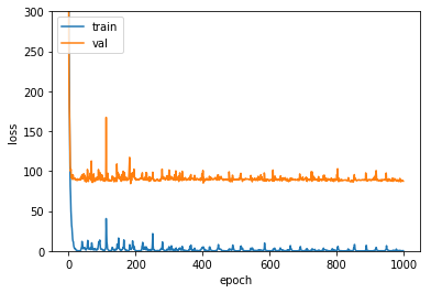 |
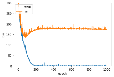 |
요약
영상를 입력하여 수치예측을 할 수 있는 깊은 다층퍼셉트론 신경망 모델, 컨볼루션 신경망 모델을 살펴보고 그 성능을 확인 해봤습니다. 영상 입력이라고 해서 컨볼루션 신경망 모델이 항상 좋은 성능이 나오는 것이 아니라는 것도 알게되었습니다. 어떤 모델이 성능이 좋게 나올지는 테스트를 해봐야 겠지만, 워낙 모델을 다양하게 구성할 수 있고 여러 파라미터를 설정할 수 있으므로, 모델을 개발하기 전 데이터 특징을 분석하고 적절한 후보 모델들을 선정하는 것을 권장드립니다.
같이 보기
- 강좌 목차
- 이전 : 수치입력 다중클래스분류 모델 레시피
- 다음 : 영상입력 이진분류 모델 레시피
책 소개
[추천사]
- 하용호님, 카카오 데이터사이언티스트 - 뜬구름같은 딥러닝 이론을 블록이라는 손에 잡히는 실체로 만져가며 알 수 있게 하고, 구현의 어려움은 케라스라는 시를 읽듯이 읽어내려 갈 수 있는 라이브러리로 풀어준다.
- 이부일님, (주)인사아트마이닝 대표 - 여행에서도 좋은 가이드가 있으면 여행지에 대한 깊은 이해로 여행이 풍성해지듯이 이 책은 딥러닝이라는 분야를 여행할 사람들에 가장 훌륭한 가이드가 되리라고 자부할 수 있다. 이 책을 통하여 딥러닝에 대해 보지 못했던 것들이 보이고, 듣지 못했던 것들이 들리고, 말하지 못했던 것들이 말해지는 경험을 하게 될 것이다.
- 이활석님, 네이버 클로바팀 - 레고 블럭에 비유하여 누구나 이해할 수 있게 쉽게 설명해 놓은 이 책은 딥러닝의 입문 도서로서 제 역할을 다 하리라 믿습니다.
- 김진중님, 야놀자 Head of STL - 복잡했던 머릿속이 맑고 깨끗해지는 효과가 있습니다.
- 이태영님, 신한은행 디지털 전략부 AI LAB - 기존의 텐서플로우를 활용했던 분들에게 바라볼 수 있는 관점의 전환점을 줄 수 있는 Mild Stone과 같은 책이다.
- 전태균님, 쎄트렉아이 - 케라스의 특징인 단순함, 확장성, 재사용성을 눈으로 쉽게 보여주기 위해 친절하게 정리된 내용이라 생각합니다.
- 유재준님, 카이스트 - 바로 적용해보고 싶지만 어디부터 시작할지 모를 때 최선의 선택입니다.