딥러닝 공부
딥러닝 관련 논문이나 오픈된 소스를 보면서 공부한 것을 공유하고자 합니다.
-
NASA FDL 2017 연구 소개
저희회사((주)인스페이스)에서 충남대학교 백마인턴쉽 과정으로 함께 하게된 박천용 인턴님의 첫과제로 조사한 내용을 공유드립니다. 주제는 NASA Frontier Development Lab에서 진행되고 있는 연구 소개입니다.

미국 NASA의 Frontier Development Lab (FDL)은 항공 기관인 Ames Research Center와 SETI에 의해 공동 운영 되고 있으며, 이들은 잠재적 위험성을 가지고 있는 소행성과 혜성으로부터 지구를 보호하는 방법을 연구하고자 인공지능을 이용하겠다고 발표하였습니다.
지난 2014년에 매년 6월 30일을 국제 소행성 날 (International Asteroid Day)로 지정하고 Near Earth Objects(NEOs)로 부터 오는 잠재적 위협에 대한 연구결과를 발표하는 연내행사를 계획하는 것으로 만들어졌습니다. 6월 30일이 선택된 이유는 1908년에 일어난 러시에 시베리아 위치한 퉁구스카에 충돌체 사건을 기념하는 날이기 때문이었기 때문입니다. 연내 기념행사는 천체물리학자이자 Queen의 리드 기타리스트인 Brian May, 그리고 영화 제작자인 Grigorij Richters의 아이디어이었습니다. NASA FDL 팀은 NASA Frontier Development Lab 2017(FDL 2017)발표를 통해 딥러닝 기반의 다양한 연구성과를 알리게 되었습니다.
1. Solar storm prediction
개요
인공지능을 사용하여 플레어를 탐지하고, 우주 비행 임무에 결정적인 태양활동 및 우주 기상 현상의 중요성을 이해합니다. 태양 자기장 complexity 분석을 수행하고, 태양 UV 이미지를 연결하기 위해 multiple CNN을 배치했습니다. 이 연구는 태양 플레어 예측의 신뢰성과 정확성을 향상시킬 수 있는 잠재력이 있음을 보여줍니다.
플레어(Flare)란?
플레어란 태양 대기에서 발생하는, 수소폭탄 수천만 개에 해당하는 격렬한 폭발을 말합니다.

태양의 플레어는 단파장의 전자기 방사선을 발생시킵니다. 이는 상층 대기의 이온화와 가열을 초래하고, GPS와 HF의 통신에 영향을 미칩니다.
FlareNet
어떻게 NOAA(기상위성)가 플레어를 예상할수 있을까요? 태양 흑점 형태와 지속성, 즉 태양이 변하지 않는 다는 것을 가정합니다. FDL팀은 전문가들 보다 최소한 한시간 빠르게 플레어의 위험을 예측하는 것을 목표로 하였습니다.
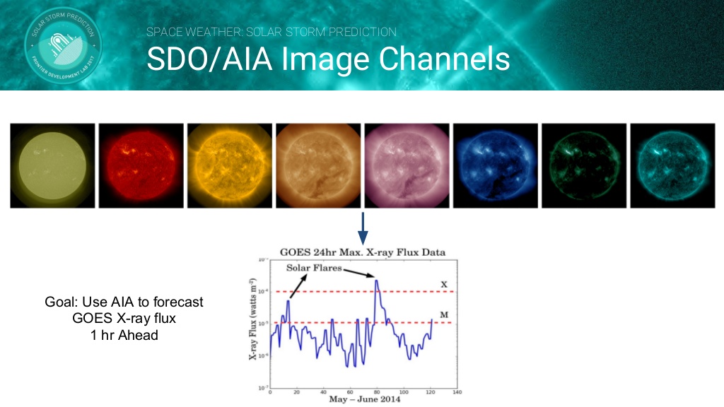
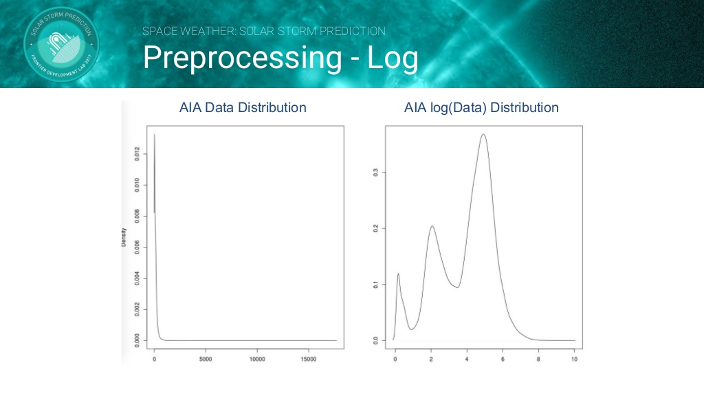
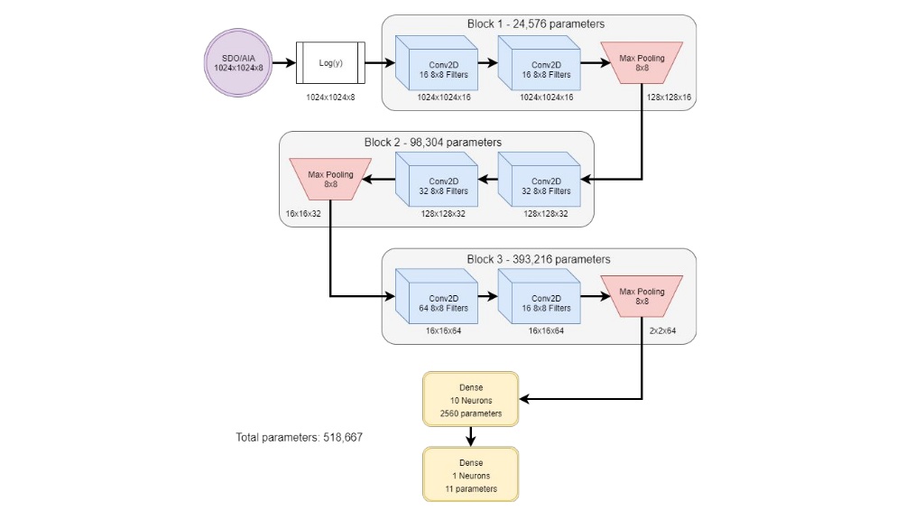
데이터셋으로는 태양의 SDO(Solar Dynamic Observatory)/AIA(Atmospheric Imaging Assembly) Image를 사용합니다. 그러나 AIA 데이터는 높은 동적 범위(High dynamic range)의 문제가 존재하기 때문에 Log Transform 을 하여 데이터를 전처리합니다. 전처리 과정을 거친 데이터를 아래의 CNN모델로 학습시킵니다.
결론
- FlareNet은 상위 수준의 X 선 플럭스 활동을 생성 할 수 있습니다.
- FlareNet은 태양의 구조 뿐만 아니라 active regions의 중요성을 학습하였습니다.
2. Long Period Comets
개요
천문학적인 유성우의 발견은 천년기에 지구 궤도를 가로지르는 긴 주기의 혜성의 존재를 암시합니다. 머신러닝과 딥러닝을 사용한 유성 분류의 자동화를 연구합니다. 유성우 관측에 기계 학습을 적용하여 오랜 기간 혜성 충돌에 대한 더 많은 경고를 제공합니다. 유성우 궤도는 예상 궤도를 따라 전용 검색을 가능하게 합니다.
CAMS
LSTM을 이용한 유성 판별
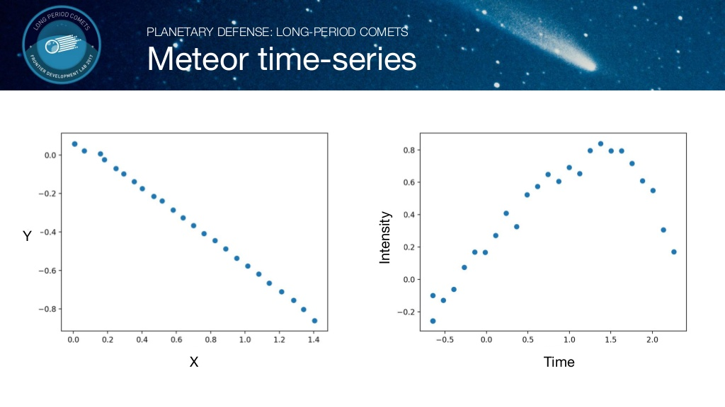
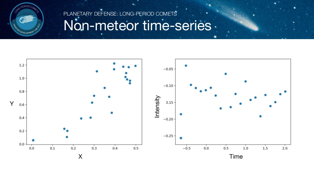
각 개체의 시간에 따른 위치를 X,Y 좌표계로 나타내고, Intensity(밝기,빛의 모양 등)를 시간에 따라 그래프로 나타내었습니다. 위 그림은 유성인 것과 유성이 아닌 것에 대한 비교 그래프입니다. 유성의 경우 규칙적인 값을 갖는 반면에, 유성이 아닌 경우 불규칙적인 값을 갖습니다.
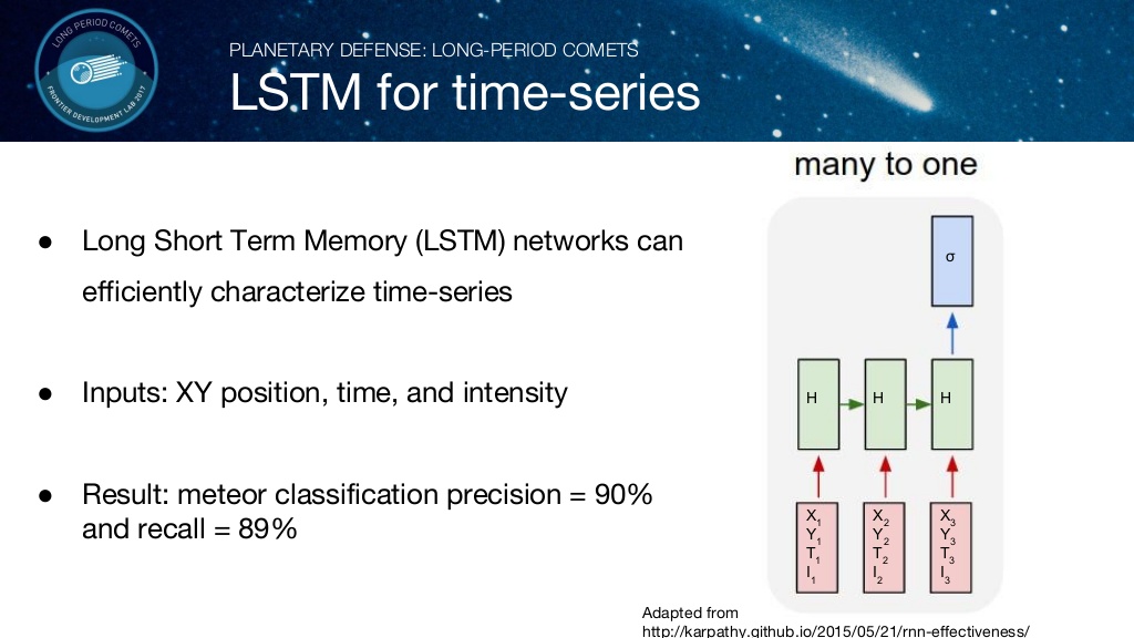
위의 Tracklets(궤도)데이타를 입력으로 하는 LSTM 모델을 활용하여 유성을 판별합니다.
CNN을 이용한 유성 판별
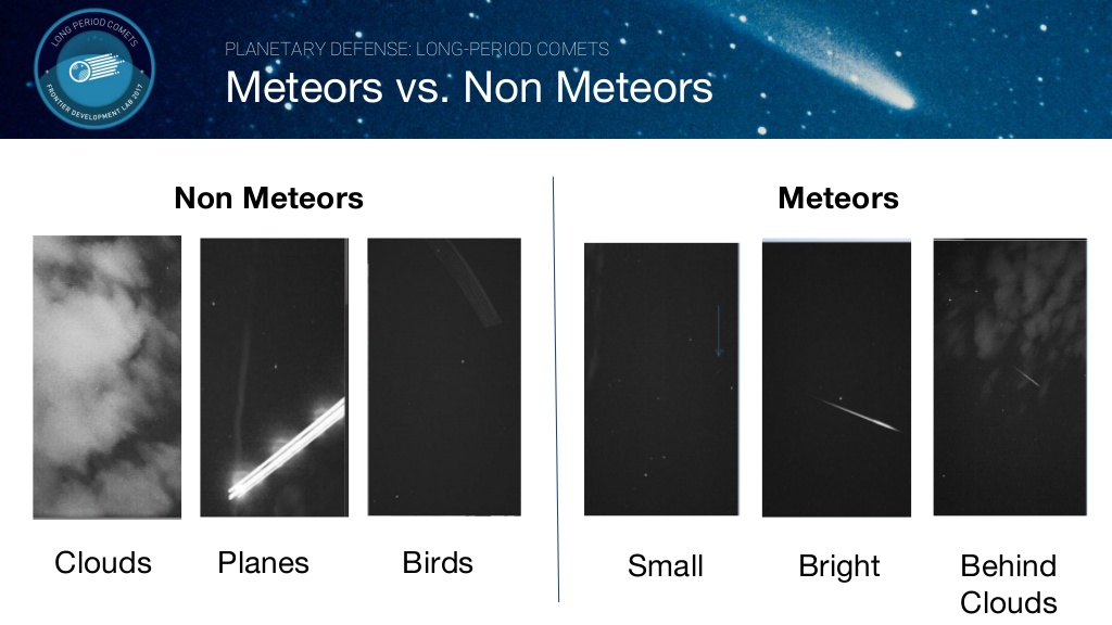
위 이미지와 같은 Label된 데이터를 바탕으로 Convolution Neural Network를 이용하여 유성 여부를 판별합니다.
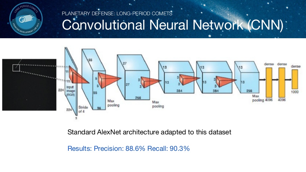
이미지를 입력으로 하는 CNN 모델을 활용하여 유성을 판별합니다.
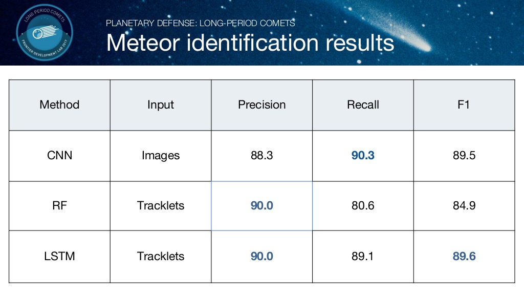
결론
다음은 각 모델 별로 정확도와 F1 스코어를 계산한 값입니다. LSTM을 사용한 모델이 F1 score가 제일 높게 나온 것을 확인 할 수 있습니다.
3. Lunar Water and Volatiles
개요
수자원이 풍부한 지역을 탐사하기 위한 crater map의 자동 제작을 연구합니다. 달의 남극에서 대규모 데이터 셋을 수집하고 크레이터 감지에 초점을 둔 고급의 feature 추출을 수행합니다. 98,4%의 높은 성공률로 전문가보다 100배 빠른 속도향상을 이루어냈습니다.
달에 물이 존재하는 곳
- 극 근처에 존재하는 크레이터
- 태양이 닿지 않는 크레이터의 바닥
- 영원히 그림자 진 지역(PSRs)

대부분의 달에 존재하는 물은 극점에 있는 PSRs에 존재합니다. 따라서 달에 존재하는 물을 찾기위해서는 먼저 PSR 및 크레이터를 연구할 필요가 있습니다. 그러나 달의 극점을 Mapping 하기위한 문제점이 존재합니다.
- Co-regstration issues
- Artifacts
- Image illumination
따라서 의미 있는 실험을 수행하기 위해서는 노동집약적인 많은 데이터가 필요합니다.
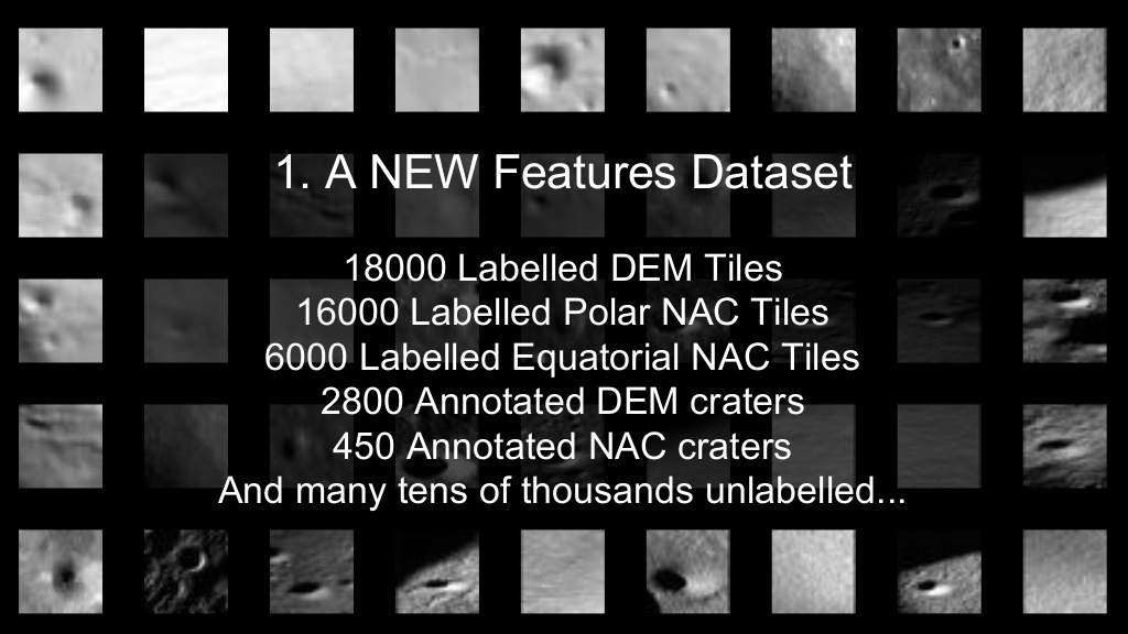
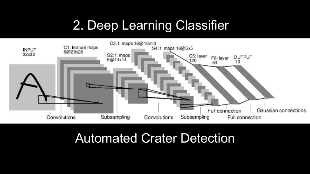
Deep Learning Classifier
달의 크레이터를 분별하기 위해서 달의 사진을 데이터 셋으로 사용합니다. 달의 DEM(Digital Elevation Model)/NAC(Narrow Angle Camera)을 Annotation 한 뒤 사용합니다. 사용된 데이터 셋의 크기는 다음과 같습니다.
Annotation 과정을 거친 데이터 셋은 CNN을 사용하는 Classifier 모델을 학습시키는 데 사용됩니다.
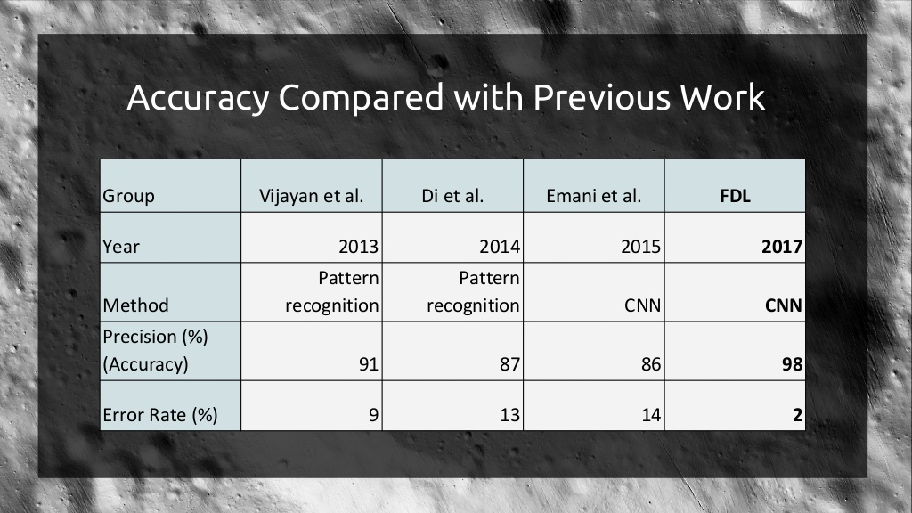
결론
FDL팀이 연구한 CNN 모델이 지난 팀들이 연구한 패턴인식을 사용한 방법이나 CNN 모델 보다 월등히 뛰어난 정확도를 보이고 있습니다.
4. Radar 3D Shape Modeling
개요
2016 년부터 작업을 계속하면서 팀은 형상 모델링 워크 플로에 따라 AI 기술을 적용했습니다. 소행체 모양 모델링은 기존 소프트웨어를 사용하는 전문가가 수동으로 개입하는 데 최대 4 주가 소요됩니다. 이 팀은 Neural Nets를 최적화하고 GAN(Generative Adversarial Nets)을 활용하여 몇 시간 내에 NEO(Near Earth Object)를 모델링 할 수있는 자동화를위한 파이프 라인을 시연했습니다.
데이터셋
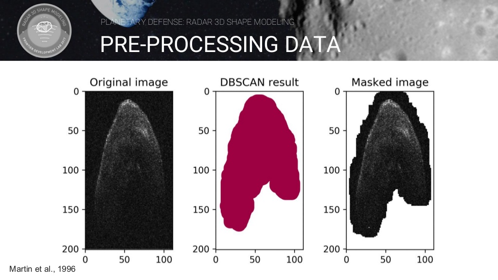
DBSCAN(Density-Based spatial clustering of applications with noise)은 주변 데이터들의 밀도를 이용해 군집을 생성해 나가는 방식을 말합니다. DBSCAN 결과에 image를 Masking 하여 이미지 데이터 전처리를 실시합니다.
GAN모델을 이용한 소행성 모델링 생성
GAN(Generative adversarial networks)이란 Generator 네트워크와 Discriminator 네트워크가 서로 경쟁하며 성능을 점차 증진시켜나가는 방식의 모델입니다.
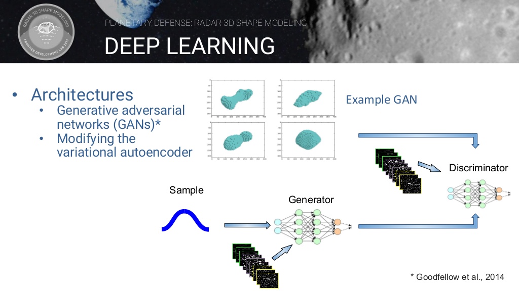
Generator에서 만들어진 모델링을 Discriminator가 판별하여 결과를 Generator에게 알려줍니다. 이를 계속 반복하면 Discriminator는 가짜를 판별하는 능력이 향상될 것이며 Generator는 실제 모델링과 비슷한 모델링을 만들어 낼 것 입니다. 두 네트워크의 경쟁을 통해 실제와 비슷한 모델링을 만들어 내는 것이 목표입니다.
5. Solar Terrestrial Interactions
개요
지구 자기권의 적도 전류링 문제를 풀면서 딥러닝 기술을 과학적인 돌파구를 위한 도구로서의 가능성을 살펴보겠습니다. 오픈 소스 시스템 학습 프레임 워크 위에 STING (Solar Terrestrial Interactions Neural Network Generator)이라는 지식 검색 모듈을 구축하여 연구자가 복잡한 데이터 세트를 더 자세히 탐색 할 수 있게 했습니다.
Space Weather가 주는 영향
“우주 환경” 혹은 “우주 기상”이라는 용어는 우리가 지구에서 사용하는 기술의 성능에 영향을 미칠 수 있는 태양과 우주에서의 변수 상태를 지칭합니다. 우주 기상은 전선의 극심한 전류를 유도하는 전자기장을 생성하여 전선을 방해하고 광범위한 정전을 일으키기도 합니다. 심각한 우주 기상은 태양 에너지 입자도 생성하여 상업용 통신, 세계 위치 파악, 정보 수집 및 기상 예보에 사용되는 위성을 손상시킬 수 있습니다 다음은 우주 기상의 예시인 오로라가 끼치는 영향을 그림으로 나타낸 것입니다.

B - Sting
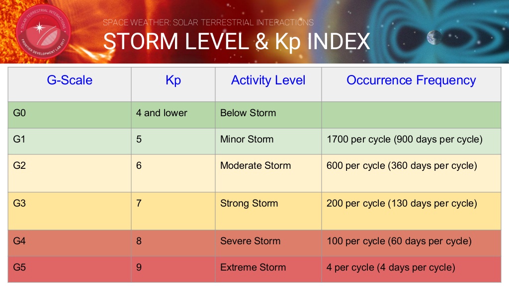
우주 일기 예보를위한 데이터 기반 오픈 소스 도구로 지자기 장애를 포착하는 Kp 지수를 예측합니다. 데이터 소스로는 지구의 자기장과 태양풍 데이터를 사용합니다. Kp 지수는 매일 3 시간 간격으로 측정 한 지자기 활동 수준의 범위를 나타냅니다.
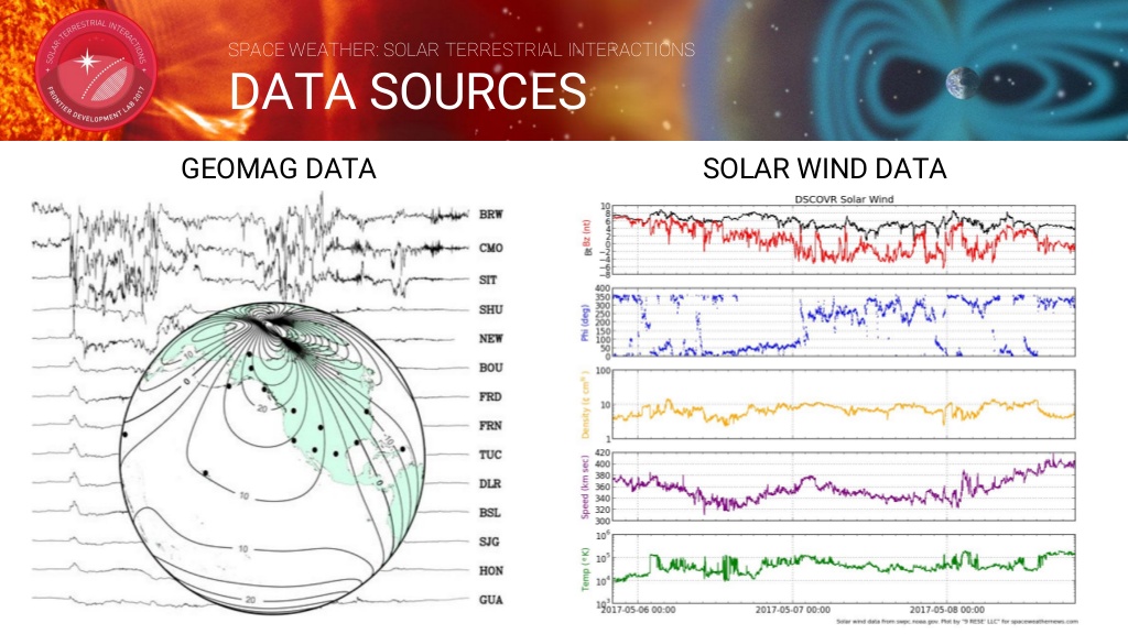
지구의 자기장과 태양풍 데이터를 입력으로 Kp지수를 측정하기 위해서 다음과 같은 두가지 프로젝트를 실시했습니다.
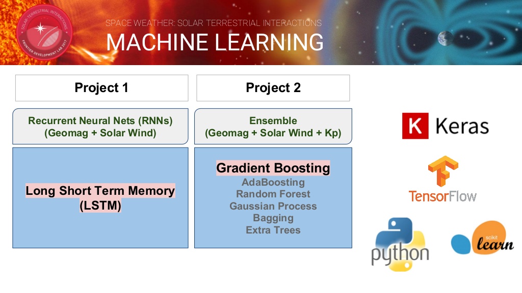
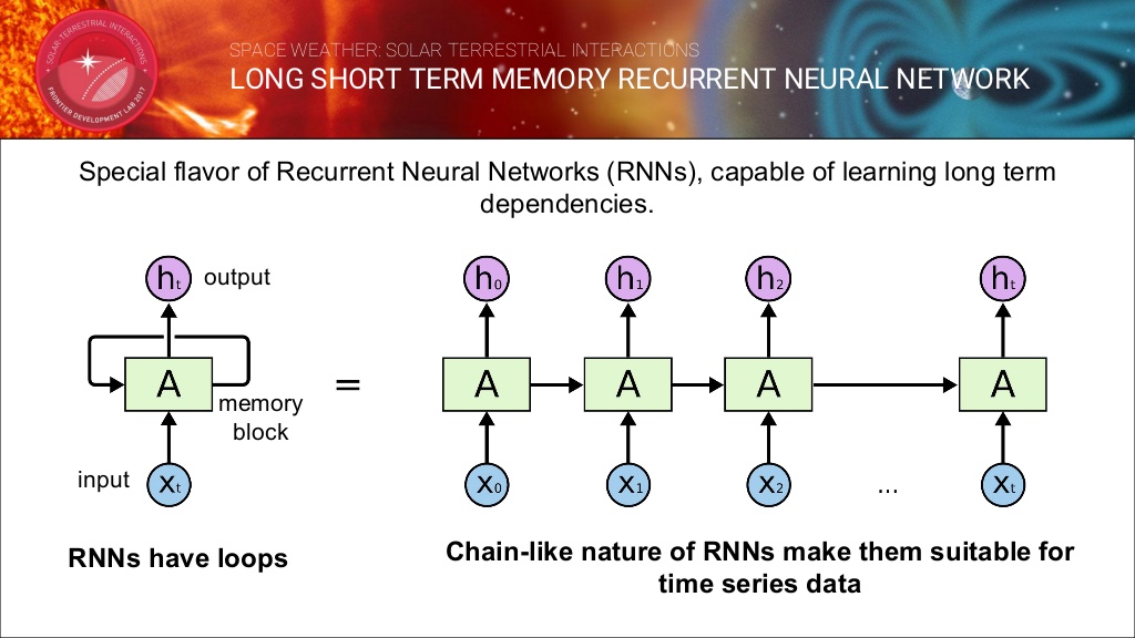
LSTM RNN 모델
LSTM유닛은 여러 개의 게이트(gate)가 붙어있는 셀(cell)로 이루어져있으며 이 셀의 정보를 새로 저장/셀의 정보를 불러오기/셀의 정보를 유지하는 기능이 있습니다. 셀은 셀에 연결된 게이트의 값을 보고 무엇을 저장할지, 언제 정보를 내보낼지, 언제 쓰고 언제 지울지를 결정합니다.
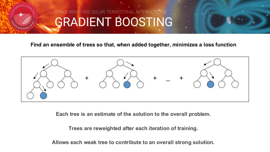
Gradient Boosting 모델
함께 합쳐지면 손실 함수가 최소화되도록 트리 앙상블을 찾습니다. 각 트리는 전반적인 문제에 대한 솔루션의 추정치입니다. 훈련이 반복 될 때마다 나무에 재사용됩니다. 각 취약한 트리가 전반적인 강력한 솔루션에 기여할 수 있게 하였습니다.
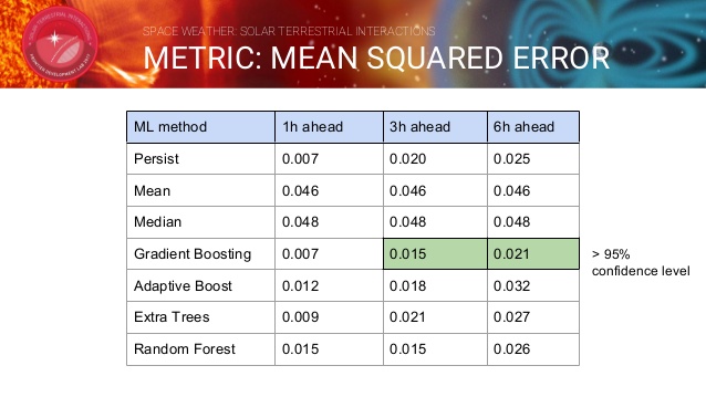
결론
다음은 Gradient Boosting 방법을 통해 3시간뒤의 Kp지수를 예측한 값과 실제 값을 비교한 그래프입니다.
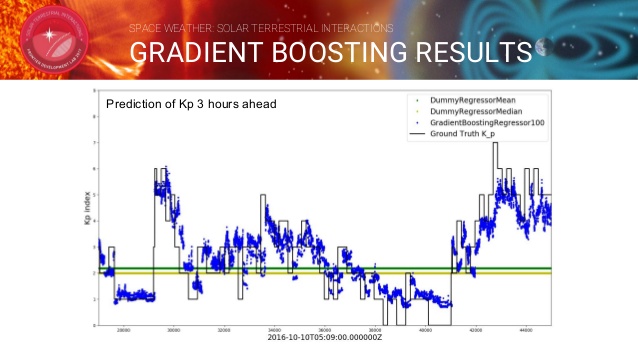
Gradient Boosting 방법을 사용한 결과가 기존에 제시한 방법들보다 95%의 정확성을 보여주면서 뛰어난 성능을 보이고 있습니다.
-
케라스 단점
케라스를 다른 분들께 추천을 하려면 장단점을 제대로 알고 소개를 해야 겠다는 생각이 들었습니다. 아래 나열된 단점은 커뮤너티에 올려진 게시물이나 주변에서 말하고나 제가 느낀 점을 정리해봤습니다. 어떤 항목들은 시간이 지나면서 해결되고 있는 부분들도 있습니다. 다른 단점이나 의견이 있으신 분들은 댓글로 달아주세요.

오류 대처의 어려움
- 코드에 오류가 발생하였을 경우 케라스 자체 에러일 수도 있고 사용한 백엔드(텐서플로우 등) 문제일 수도 있기에 원인 찾기가 쉽지 않습니다.
- 오류에 대한 조언을 얻기 위해 커뮤너티를 활용할 경우에도 백엔드(텐서플로우 등) 커뮤너티나 케라스 커뮤너티 모두 도움을 요청해야하는 일이 발생할 수 있습니다.
- 만약 케라스에 오류가 있거나 지원되지 않는 기능을 직접 수정한다고 했을 때, 케라스 코드를 수정할 수 있습니다만 케라스 인터페이스에 맞추어서 수정하는 것보다 그냥 벡엔드를 익혀서 수정하는 것이 더 빠를 수 있습니다.
참고할 때가 부족
- 문서화가 제대로 되어 있지 않습니다. 제공되는 함수 목록은 빨리 업데이트 되는 편이지만 함수에 대한 설명을 찾기란 쉽지 않습니다.
- 충분한 공식 예제가 없습니다. 케라스로 만든 예제들은 많지만 공식적으로 제공되는 예제는 한정적입니다.
- 한국에서 사용자가 적어 물어볼 곳이 마땅히 없습니다.
한정적인 기능 제공
- 케라스에서 제공하는 텍스트 및 이미지 전처리 기능을 제공하지만 다양한 전처리를 원한다면 다른 패키지(scikit-learn이나 pandas 등)을 사용해야 됩니다.
단점을 보안하고자 하는 노력들 (한국에서)
- 케라스를 주요 주제로한 페이스북 그룹인 케라스 코리아가 있습니다. 이 그룹을 통해서 한국에서 사용자 층을 늘리고, 자유롭게 질문과 답을 할 수 있는 장을 만들고자 합니다.
- 케라스를 주제로 한 국내 도서들이 발간되고 있습니다. 저자가 이끄는 가이드대로 차근차근 공부하시고 싶은 분들은 도서를 추천합니다.
- 2017년 7월 파이썬과 케라스로 배우는 강화학습
- 2017년 8월 블록과 함께하는 파이썬 딥러닝 케라스
- 2018년 1월 코딩셰프의 3분 딥러닝, 케라스맛
-
한 장 간
제 마음대로 ‘네트워크’와 ‘모델’을 구분해서 개념 정리를 해본 것을 그림으로 표현해봤습니다.

이 그림을 그리게 된 계기가 있는데요. 케라스의 GAN 코드를 보다가 엄청 헷갈리는 부분이 있었는데 이것 때문에 개념삽질 좀 했습니다. 그 부분은 바로 “discriminator.trainable = False” 이것입니다. 일단 대부분의 GAN 코드는 다음과 같은 구성을 가지고 있습니다.
# generator 생성
generator = Sequential()
generator.add(...)
generator.compile(...)

# discriminator 생성
discriminator = Sequential()
discriminator.add(...)
discriminator.compile(...)

# adversarial network 생성
discriminator.trainable = False ## << 바로 이부분
gan_in = Input(shape=(randomDim,))
gan_out = discriminator(generator(gan_in))
gan = Model(inputs=gan_in, outputs=gan_out)
gan.compile(...)
discriminator 학습 시킬 때는 참/거짓 데이터를 주고 가중치를 업데이트를 해야되지만, 이 discriminator가 gan 안에서 generator와 같이 학습할 때는 가중치가 고정되어 있어야 합니다. 그래서 gan 모델을 생성하기 전에 discriminator.trainable = False으로 설정하긴 했는데… 여기서 헷갈리기 시작했습니다.
- discriminator.trainable = False 으로 하면 gan에서는 고정되겠지만 discriminator을 학습할 때도 가중치가 고정되는 것이 아니야?
- 앞에서 생성한 discriminator과 gan에 삽입할 때의 discriminator는 다른 객체인가?
등등으로 생각을 했었는데, 알고보니 compile() 함수가 호출될 때 trainable 속성이 모델에 적용되더라구요. 즉 다음과 같습니다.
- discriminator을 생성한 뒤 compile() 하면 trainable = True로 컴파일 됨
- discriminator.trainable = False으로 적용하면 일단 trainable 속성만 비활성화된 상태임
- gan 모델에 discriminator가 삽입됨
- gan.compile() 하면 gan 모델 안에서 discriminator의 가중치가 업데이트 되지 않음
- gan.compile()과 discriminator.compile()은 별개이고, discriminator.compile()가 다시 호출 되지 않았으므로, discriminator 모델에서의 trainable 속성은 True임
- 여기서 하나 알 수 있는 것은 discriminator이라는 네트워크는 discriminator 모델과 gan 모델에 둘 다 사용되고 가중치도 공유되나 discriminator 모델에서는 가중치 갱신이 일어나고, gan 모델에서는 가중치 갱신이 일어나지 않음
- gan 모델에서의 discriminator 네트워크는 단순 가중치를 가진 네트워크로만 받아들이고 discriminator 모델에 적용된 compile()은 아무 영향을 주지 않음. 즉 gan 모델은 따로 complie()을 해야 함
배성호교수님의 ‘간은 로스일 뿐이야’라는 말씀을 이제야 이해한 듯 합니다.
같이 보기
-
딥브릭(DeepBrick) 이야기
딥러닝과 케라스를 공부하면서 느낀 점은 층을 쌓고 모델을 만들고 하는 과정들이 블록 쌓는 것과 비슷한 느낌을 많이 받았고, 실제로 딥러닝 모델을 설명할 때 블록 그림을 많이 이용하기도 했습니다. 그러다가 (실제 혹은 웹에서) 블록을 쌓으면 딥러닝 모델까지 자동으로 만들 수 있겠다는 생각이 들었습니다. 그래서
딥브릭(DeepBrick)이란 이름으로 프로젝트를 진행해볼까 합니다.
유닛
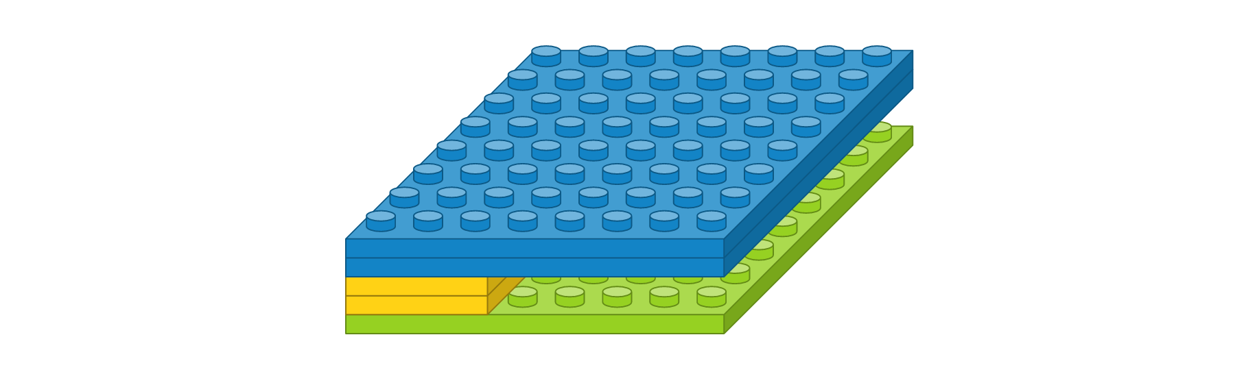
딥러닝 모델에서의 개념과 우리가 익숙한 블록 간이 연관성이 있다록 매칭하는 작업이 필요했습니다. 지금까지 정리된 컨셉은 다음 그림과 같습니다.
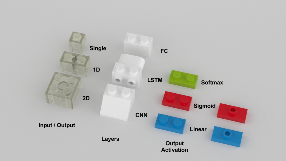
- 투명한 블록은 입출력을 나타냅니다. 22 블록은 이미지를 의미하고, 12는 두개 이상 값을 가지는 백터, 1*1는 한 개 값을 가지는 벡터입니다.
- 흰 블록은 모델을 의미합니다. 현재 모델은 CNN, LSTM, FC 이렇게 3가지 구상해봤습니다. 만약 프로그램을 만든다면 이 블록을 우클릭하면 층, 파라미터를 설정하거나 스크립트가 열리는 식이겠죠?
- 얇은 블록은 출력을 정의합니다. Softmax는 다중분류 문제 사용되고, Sigmoid는 이진분류 또는 회귀문제, Linear는 회귀문제에 사용됩니다.
동영상 분류 문제
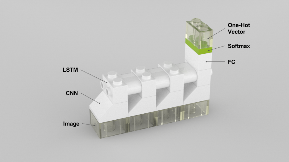
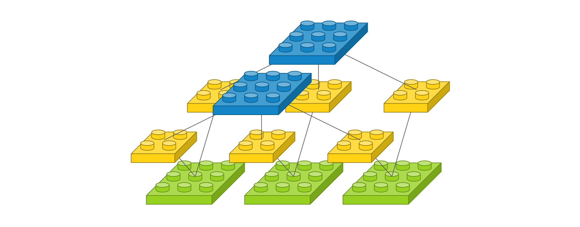
위에서 정의한 유닛을 이용해서 동영상 분류 문제를 풀기 위해 CNN + LSTM을 이용해서 모델 하나를 만들어봤습니다.
- 입력은 이미지라서 2D 투명 블록으로,
- 이미지를 인코딩하기 위해 입력은 CNN 블록으로,
- 시계열 이미지(동영상, 4 프레임)를 처리하기 위해 LSTM 블록을 위에 얹히고,
- 마지막 LSTM 블록에 FC 블록을 연결한 다음 Softmax 블록을 쌓았습니다.
- Softmax 블록 위에 출력 1D 투명 블록을 쌓아서 출력을 얻습니다.
- 이 출력은 one-hot 벡터입니다.
이 모델에 해당하는 케라스 코드도 같이 작성해봤습니다.
model = Sequential()

# CNN
model.add(TimeDistributed(Conv2D(32, (2, 2), activation='relu'), input_shape=(None, 32, 32, 1)))
model.add(TimeDistributed(MaxPooling2D(pool_size=(2,2))))
model.add(TimeDistributed(Flatten()))

# LSTM
model.add(LSTM(128))

# FC
model.add(Dense(2, activation='softmax'))

# Compile
model.compile(loss='categorical_crossentropy', optimizer='adam', metrics=['acc'])
코드 생성 모듈 개발하시는 분들이 보시기엔 어떻게 느껴지실 지 궁금합니다. ‘할 만 하겠어’라고 생각하시겠죠? 이제(아니 나중에…) 블록만 조립하면 케라스 코드가 자동 생성됩니다.
블록 이야기
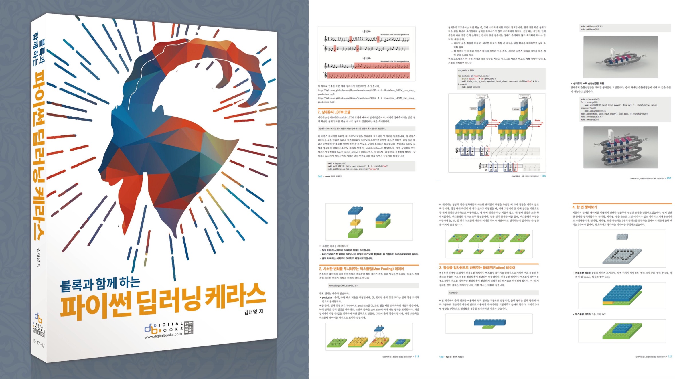
블록으로 표시하기 위한 고민을 많이 해왔습니다. 처음에는 레고로 조립해서 사진으로 찍었었는데, 원하는 부품을 구하기도 힘들뿐더러 (정확히는 돈이 많이 듭니다) 찍어도 그리 예쁘지가 않았습니다. 그 다음에 고민한 것이 블록 생성 툴을 알아봤었는 데, 원하는 품질이 나오지 않아 구글 프리젠테이션으로 직접 그리게 되었습니다(아래 그림에서 왼쪽). 하나 하나 다 그려야 되서 손이 많이 가긴 했었는데, 나름 편해서 잘 쓰고 있었습니다. 그러다 좀 다양한 블록을 표현하고 싶은데 구글 프리젠테이션으론 더 이상 할 수 없다는 결론을 내리고 다시 툴을 찾기 시작했습니다. 그러다 “Mecabricks”와 “blender” 툴의 조합으로 아래 그림에서 오른쪽으로 표현할 수 있게 되었습니다. 상상 이상의 고퀄이라 부담스러울 정도긴 한데, 손으로 일일이 그리는 것 보단 100배 편해서 사용하기로 결정했습니다. 나중에 알아보니 레고 영화 제작할 때 사용한다고도 하더군요.
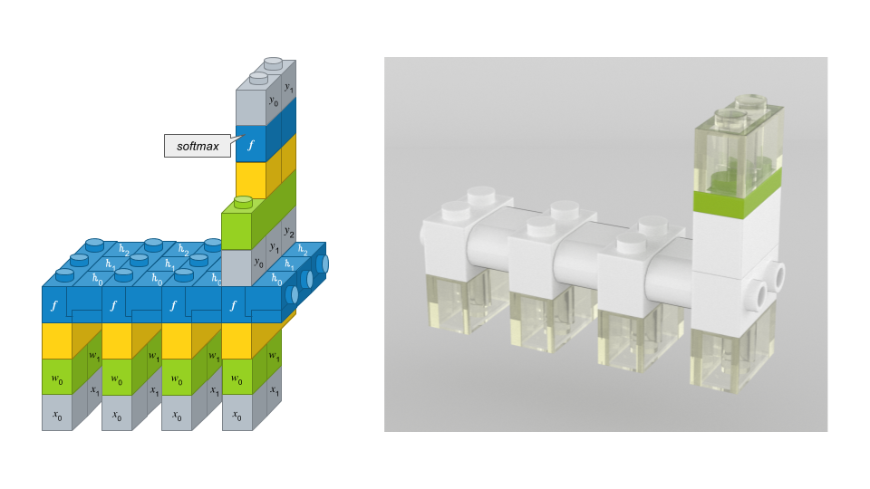
두 개 버전을 비교하면 좀 더 추상화가 되어 간단해졌고, 실사에 가깝게 되었습니다~ 블록 표시하는 것에 대해서는 갈때까지 간 것 같습니다.
결론
저는 상상이되는 글, 그림, 코드, 생각 등을 좋아합니다. 이 이야기는 상당히 상상력이 자극되는 것 같습니다. 얼마나 다양한 유닛이 만들어질지, 얼마나 멋진 모델을 조립할 수 있을 지 궁금하네요. 이런 상상도 해봅니다. 어린이들이 딥러닝 블록을 조립한 뒤 학습을 시키면, 그 학습 결과가 가중치 블록에 저장됩니다. 그 가중치 블록을 로봇 등이 꼽기만 하면 동작이 될 수 있겠죠? 망상에 가까울려나요? 여러 사람들의 의견으로 좀 더 직관적이고 재미있는 아이디어가 많이 담긴
딥브릭(DeepBrick) 이야기가 되었으면 합니다.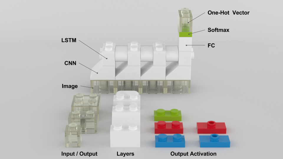
같이 보기
-
Relation Networks for Visual QA
Visual QA 문제에서 관계형 추론(relational reasoning)을 도출하고자 DeepMind가 제안한 신경망 모델인
관계 네트워크(Relation Networks, 이하 RN)대해서 알아보고자 합니다. 이 모델은 A simple neural network module for relational reasoning이란 논문에서 소개되었고, 컨볼루션 신경망에 RN를 추가하여 어떻게 객체와 그 관계에 대해 추론하는 지 설명되어 있습니다. 시각기반의 질의응답 문제에 대해 탁월한 성능을 보이고 있다고 합니다.
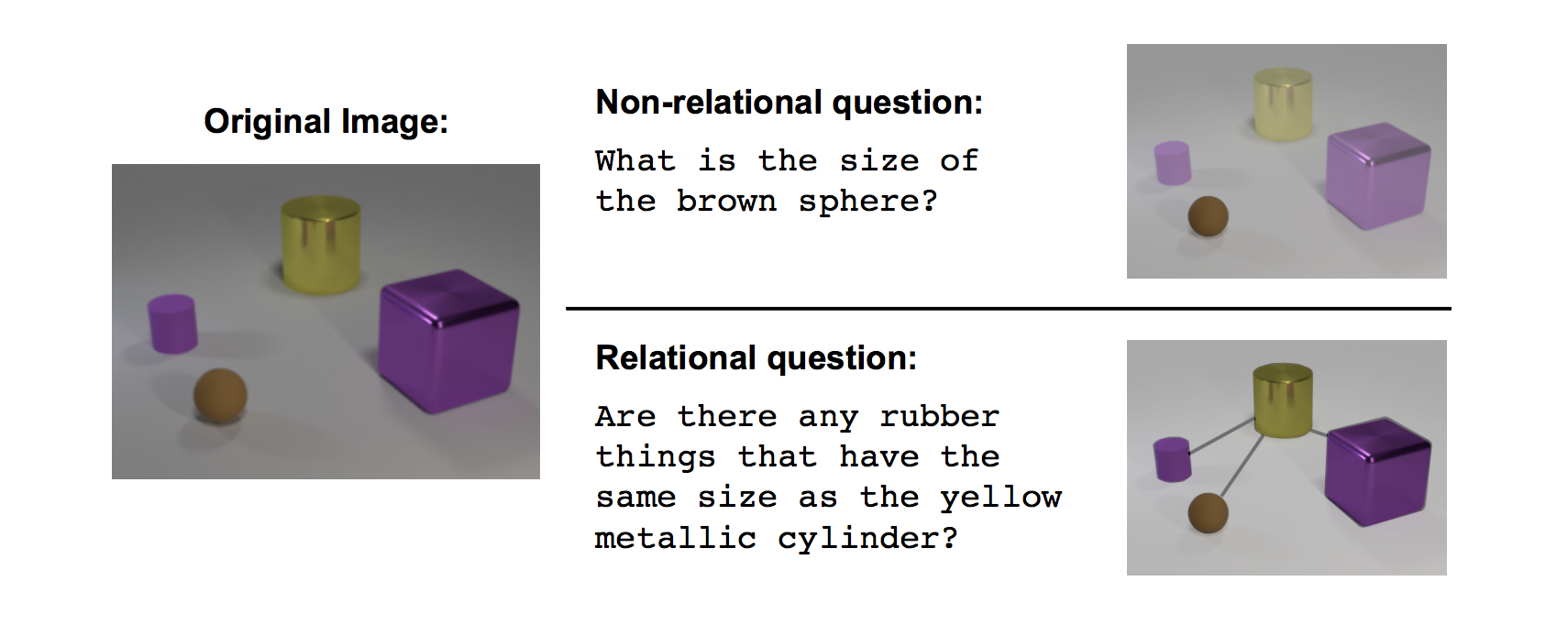
관계형 추론이란
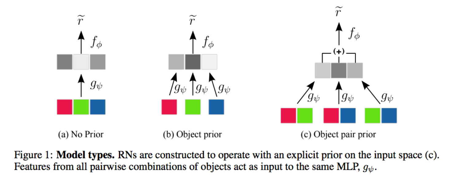
관계형 추론(Relational Reasoning)이란 객체와 객체 속성 간의 관계를 추론하는 능력입니다. 아래 그림을 보면 두가지 질문이 있는데, 특정 객체의 속성을 추론하는 것을 비관계형 질문이라고 하고, 객체 간의 관계에 대해서 추론하는 것을 관계형 질문이라고 합니다.
(Ref, arXiv:1706.01427)
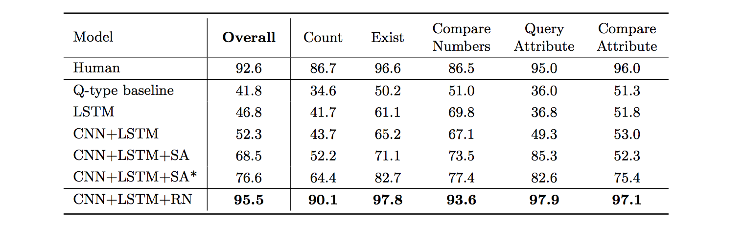
관계 네트워크(Relation Networks, RN)
DeepMind에서는 이러한 관계형 추론을 할 수 있는 RN을 개발하였습니다. RN은 간단하며, 다른 모델에 쉽게 붙일 수 있고, 유연한 관계형 추론에만 중점을 둘 수 있습니다. RN을 CNN과 LSTM과 결합하여 (본문에서는 RN-augmented architecture라고 표현) visual question answering 문제에 대해서 실험을 하였고, 좋은 결과(기존 모델은 76.6%, 사람이 92.6%, RN 모델 적용한 것이 95.5%)가 나왔다고 합니다.
(Ref, arXiv:1706.01427)
RN-augmented Visual QA acrhitecture
RN 모델 자체는 객체 관계만 추론하기 때문에 이미지나 자연어에 대해서는 동작하지 않습니다. 그래서 CNN과 LSTM 등과의 모델에서의 출력을 입력받아 객체를 추출하고 각 객체간의 관계를 추론합니다. 즉 객체를 따로 지정할 필요도 없다고 합니다. 아래는 논문에서 사용한 모델 구성입니다.
(Ref, arXiv:1706.01427)
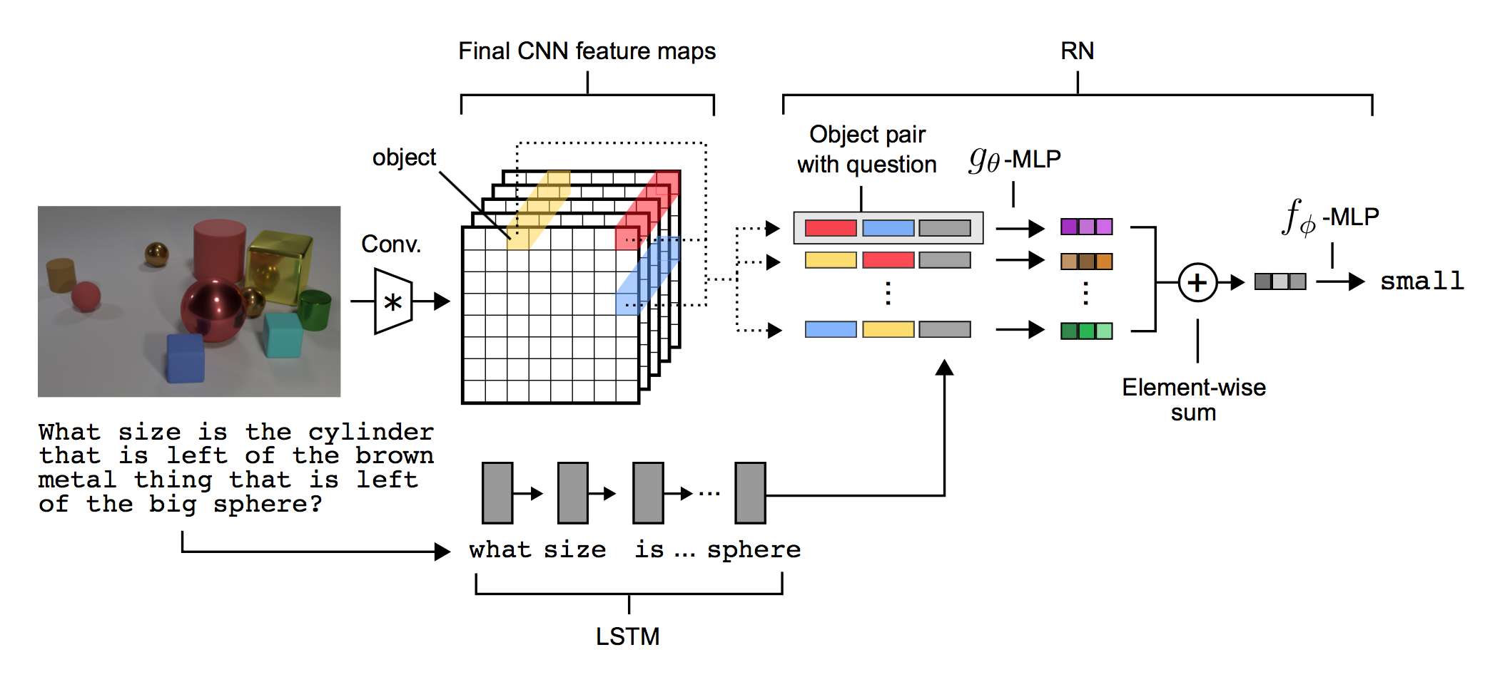
입력되는 이미지의 픽셀에서 객체들을 추출하기 위해 CNN이 사용하였습니다. 4개의 컨볼루션 레이어를 통해 크기 d * d의 k개의 feature map이 생성됩니다. k는 최종 컨볼루션 레이어의 커널 수입니다. 총 셀의 개수는 ddk가 되는 데, 각 셀은 RN에 대한 객체로 간주되며, 객체는 배경, 특정 객체, 질감, 연결 등을 정보를 담고 있습니다. 이러한 객체 정보는 인코딩된 질문과 함께 RN 모델의 입력이 됩니다.
Implementation
본 스터디에서는 Alan-Lee123 사이트에서 구현된 케라스 코드를 실행시키면서 분석해보겠습니다. 사용된 데이터셋은 Cornell NLVR이라고 불리는 시각기반의 질의응답 데이터셋입니다. 소스 구동하기 위해 아래 몇가지 사안에 대해서 고려해야 합니다.
- 백그라운드는 Tensorflow를 사용해야 함
- 버전에 따라 keras.preprocessing.text.text_to_word_sequence 함수를 재정의해야할 필요가 있음
데이터 전처리
이미지, 질문 등의 데이터를 처리하기 위한 함수 및 객체를 정의합니다.
import json
import numpy as np
import os
from PIL import Image
from keras.layers import Embedding
from keras.preprocessing.text import Tokenizer
from keras.preprocessing.sequence import pad_sequences

# text_to_word_sequence 부분에 패치가 필요하여, text_to_word_sequence 함수를 재정의함
import keras.preprocessing.text

def text_to_word_sequence(text,
                          filters='!"#$%&()*+,-./:;<=>?@[\\]^_`{|}~\t\n',
                          lower=True, split=" "):
    if lower: text = text.lower()
    if type(text) == unicode:
        translate_table = {ord(c): ord(t) for c,t in zip(filters, split*len(filters)) }
    else:
        translate_table = maketrans(filters, split * len(filters))
    text = text.translate(translate_table)
    seq = text.split(split)
    return [i for i in seq if i]

keras.preprocessing.text.text_to_word_sequence = text_to_word_sequence

EMBEDDING_DIM = 50
tokenizer = Tokenizer()

def load_data(path):
    f = open(path, 'r')
    data = []
    for l in f:
        jn = json.loads(l)
        s = jn['sentence']
        idn = jn['identifier']
        la = int(jn['label'] == 'true')
        data.append([idn, s, la])
    return data

def init_tokenizer(sdata):
    texts = [t[1] for t in sdata]
    tokenizer.fit_on_texts(texts)

def tokenize_data(sdata, mxlen):
    texts = [t[1] for t in sdata]
    seqs = tokenizer.texts_to_sequences(texts)
    seqs = pad_sequences(seqs, mxlen)
    data = {}
    for k in range(len(sdata)):
        data[sdata[k][0]] = [seqs[k], sdata[k][2]]
    return data

def load_images(path, sdata, debug=False):
    data = {}
    cnt = 0
    N = 1000
    for lists in os.listdir(path):
        p = os.path.join(path, lists)

        if not os.path.isdir(p): # 자동으로 생성되는 시스템 파일이 있을 경우 오류가 발생하기 때문에, 폴더인지 체크함
            continue

        for f in os.listdir(p):
            cnt += 1
            if debug and cnt > N:
                break
            im_path = os.path.join(p, f)
            im = Image.open(im_path)
            im = im.convert('RGB')
            im = im.resize((200, 50))
            im = np.array(im)
            idf = f[f.find('-') + 1:f.rfind('-')]
            data[f] = [im] + sdata[idf]
    ims, ws, labels = [], [], []
    for key in data:
        ims.append(data[key][0])
        ws.append(data[key][1])
        labels.append(data[key][2])
    data.clear()
    idx = np.arange(0, len(ims), 1)
    np.random.shuffle(idx)
    ims = [ims[t] for t in idx]
    ws = [ws[t] for t in idx]
    labels = [labels[t] for t in idx]
    ims = np.array(ims, dtype=np.float32)
    ws = np.array(ws, dtype=np.float32)
    labels = np.array(labels, dtype=np.float32)
    return ims, ws, labels

def get_embeddings_index():
    embeddings_index = {}
    path = './warehouse/word2vec/glove.6B.50d.txt'
    f = open(path, 'r')#, errors='ignore')
    for line in f:
        values = line.split()
        word = values[0]
        coefs = np.asarray(values[1:], dtype='float32')
        embeddings_index[word] = coefs
    f.close()
    return embeddings_index


def get_embedding_matrix(word_index, embeddings_index):
    embedding_matrix = np.zeros((len(word_index) + 1, EMBEDDING_DIM))
    for word, i in word_index.items():
        embedding_vector = embeddings_index.get(word)
        if embedding_vector is not None:
            # words not found in embedding index will be all-zeros.
            embedding_matrix[i] = embedding_vector
    return embedding_matrix
Using TensorFlow backend.데이터 로딩
앞서 정의한 전처리 함수를 이용하여 이미지 및 질문 데이터를 로딩합니다.
import numpy as np
import keras
from keras.models import Sequential, Model
from keras.layers import Dense, Dropout, Activation, Flatten, Input, Embedding, LSTM, Bidirectional, Lambda, Concatenate, Add
from keras.layers.convolutional import Conv2D, MaxPooling2D, AveragePooling2D
from keras.layers.normalization import BatchNormalization, regularizers
from keras.optimizers import Adam, RMSprop
import gc

import subprocess
import pickle

mxlen = 32
embedding_dim = 50
lstm_unit = 64
MLP_unit = 128
epochs = 50
batch_size = 256
l2_norm = 0.01

train_json = './warehouse/nlvr/train/train.json'
train_img_folder = './warehouse/nlvr/train/images'
test_json = './warehouse/nlvr/dev/dev.json'
test_img_folder = './warehouse/nlvr/dev/images'

data = load_data(train_json)
init_tokenizer(data)
data = tokenize_data(data, mxlen)
imgs, ws, labels = load_images(train_img_folder, data)
data.clear()

test_data = load_data(test_json)
test_data = tokenize_data(test_data, mxlen)
test_imgs, test_ws, test_labels = load_images(test_img_folder, test_data)
test_data.clear()

imgs_mean = np.mean(imgs)
imgs_std = np.std(imgs - imgs_mean)
imgs = (imgs - imgs_mean) / imgs_std

test_imgs = (test_imgs - imgs_mean) / imgs_std
CNN 및 LSTM 모델 구성
이미지를 처리하기 위한 CNN과 질문을 처리하기 위한 LSTM 모델을 정의합니다.
def embedding_layer(word_index, embedding_index, sequence_len):
    embedding_matrix = get_embedding_matrix(word_index, embedding_index)
    return Embedding(len(word_index) + 1,
                     EMBEDDING_DIM,
                     weights=[embedding_matrix],
                     input_length=sequence_len,
                     trainable=False)

def bn_layer(x, conv_unit):
    def f(inputs):
        md = Conv2D(x, (conv_unit, conv_unit), padding='same', kernel_initializer='he_normal')(inputs)
        md = BatchNormalization()(md)
        return Activation('relu')(md)

    return f

def conv_net(inputs):
    model = bn_layer(16, 3)(inputs)
    model = MaxPooling2D((4, 4), 4)(model)
    model = bn_layer(16, 3)(model)
    model = MaxPooling2D((3, 3), 3)(model)
    model = bn_layer(16, 3)(model)
    model = MaxPooling2D((2, 2), 2)(model)
    model = bn_layer(32, 3)(model)
    return model
input1 = Input((50, 200, 3)) input2 = Input((mxlen,)) cnn_features = conv_net(input1) embedding_layer = embedding_layer(tokenizer.word_index, get_embeddings_index(), mxlen) embedding = embedding_layer(input2) # embedding = Embedding(mxlen, embedding_dim)(input2) bi_lstm = Bidirectional(LSTM(lstm_unit, implementation=2, return_sequences=False, recurrent_regularizer=regularizers.l2(l2_norm), recurrent_dropout=0.25)) lstm_encode = bi_lstm(embedding) shapes = cnn_features.shape w, h = shapes[1], shapes[2]RN 모델 구성
CNN을 통해서 나온 feature map을 행과 열로 짤라서, Bi-LSTM으로 인코딩된 질문과 관계를 형성한 뒤 이를 dense 레이어로 구성합니다.
def slice_1(t):
    return t[:, 0, :, :]

def slice_2(t):
    return t[:, 1:, :, :]

def slice_3(t):
    return t[:, 0, :]

def slice_4(t):
    return t[:, 1:, :]

slice_layer1 = Lambda(slice_1)
slice_layer2 = Lambda(slice_2)
slice_layer3 = Lambda(slice_3)
slice_layer4 = Lambda(slice_4)

features = []
for k1 in range(w):
    features1 = slice_layer1(cnn_features)
    cnn_features = slice_layer2(cnn_features)
    for k2 in range(h):
        features2 = slice_layer3(features1)
        features1 = slice_layer4(features1)
        features.append(features2)

relations = []
concat = Concatenate()
for feature1 in features:
    for feature2 in features:
        relations.append(concat([feature1, feature2, lstm_encode]))

def stack_layer(layers):
    def f(x):
        for k in range(len(layers)):
            x = layers[k](x)
        return x
    return f

def get_MLP(n):
    r = []
    for k in range(n):
        s = stack_layer([
            Dense(MLP_unit),
            BatchNormalization(),
            Activation('relu')
        ])
        r.append(s)
    return stack_layer(r)

def bn_dense(x):
    y = Dense(MLP_unit)(x)
    y = BatchNormalization()(y)
    y = Activation('relu')(y)
    y = Dropout(0.5)(y)
    return y

g_MLP = get_MLP(3)

mid_relations = []
for r in relations:
    mid_relations.append(g_MLP(r))
combined_relation = Add()(mid_relations)

rn = bn_dense(combined_relation)
rn = bn_dense(rn)
pred = Dense(1, activation='sigmoid')(rn)
구성하는 과정이 조금 복잡할 수 있는데, 2017년 2월에 나왔던 아래 논문을 보면 RN에 대해서 좀 더 상세하게 설명되었습니다.
(Ref, arXiv:1702.05068)
모델 조합
지금까지 만든 모델을 조합합니다.
model = Model(inputs=[input1, input2], outputs=pred)
optimizer = Adam(lr=3e-4)
model.compile(optimizer=optimizer, loss='binary_crossentropy', metrics=['accuracy'])
from IPython.display import SVG from keras.utils.vis_utils import model_to_dot %matplotlib inline SVG(model_to_dot(model, show_shapes=True).create(prog='dot', format='svg'))아래 그림은 구성된 모델을 도식화 한 것입니다. 잘 확대해서 보시기 바랍니다.

모델 학습하기
구성된 모델을 훈련셋으로 학습합니다. 검증셋은 시험셋으로 사용하였네요.
model.fit([imgs, ws], labels, validation_data=[[test_imgs, test_ws], test_labels], epochs=epochs, batch_size=batch_size)Train on 74460 samples, validate on 5934 samples Epoch 1/50 74460/74460 [==============================] - 3981s - loss: 1.0313 - acc: 0.5506 - val_loss: 0.7847 - val_acc: 0.5484 Epoch 2/50 74460/74460 [==============================] - 1255s - loss: 0.7153 - acc: 0.5630 - val_loss: 0.6877 - val_acc: 0.5425 Epoch 3/50 74460/74460 [==============================] - 1027s - loss: 0.6576 - acc: 0.5740 - val_loss: 0.6664 - val_acc: 0.5693 Epoch 4/50 74460/74460 [==============================] - 1015s - loss: 0.6421 - acc: 0.5805 - val_loss: 0.6624 - val_acc: 0.5644 Epoch 5/50 74460/74460 [==============================] - 1021s - loss: 0.6343 - acc: 0.5920 - val_loss: 0.6584 - val_acc: 0.5797 ... Epoch 46/50 74460/74460 [==============================] - 1016s - loss: 0.1855 - acc: 0.9210 - val_loss: 3.5557 - val_acc: 0.5121 Epoch 47/50 74460/74460 [==============================] - 1018s - loss: 0.1775 - acc: 0.9240 - val_loss: 4.1076 - val_acc: 0.4949 Epoch 48/50 74460/74460 [==============================] - 1021s - loss: 0.1716 - acc: 0.9282 - val_loss: 3.0868 - val_acc: 0.5300 Epoch 49/50 74460/74460 [==============================] - 1027s - loss: 0.1699 - acc: 0.9279 - val_loss: 3.1258 - val_acc: 0.5153 Epoch 50/50 74460/74460 [==============================] - 1020s - loss: 0.1673 - acc: 0.9305 - val_loss: 3.3528 - val_acc: 0.5163평가
훈련 정확도는 93%이상이나 시험셋으로 평가했을 때는 51% 정도 나왔습니다.
### Test scores = model.evaluate([test_imgs, test_ws], test_labels, batch_size=128) print("%s: %.2f%%" % (model.metrics_names[1], scores[1]*100))5934/5934 [==============================] - 40s acc: 51.63%
결론
상당히 오버피팅이 되었는데, 무슨 이유인지 차근히 살펴봐야겠습니다. 참고로 Pytorch로 구현된 코드도 보입니다. 여기서는 결과가 관계형 질문 정확도가 89%, 비관계형 질문 정확도가 99%이라고 되어있네요.
같은 시기에 DeepMind에서 Visual Interaction Networks이란 논문도 나왔습니다. 아래 그림을 보시면 6 프레임을 입력하여 200프레임을 예측한 결과인데, 상당히 잘 맞습니다.
(Ref, DeepMind)
Visual Interaction Network는 시각적 모듈과 물리적 추론 모듈의 두 가지 메커니즘으로 구성되며, 시각적 장면 처리는 물론 미래에 어떤 일이 일어날 지 예측할 수있는 암묵적 시스템 규칙(예를 들어 물리 시스템)을 학습한다고 합니다. 현상만 잘 학습시키면, 딥러닝 기반의 물리 엔진이 만들어질 기세입니다. 다양한 활용 사례를 기대해봅니다.
같이 보기
-
파이썬 패키지 이야기
딥러닝 모델 개발에 유용한 파이썬 패키지에 대해서 다뤄봅니다.
Pickle
users = {'id1':'kim', 'id2':'lee', 'id3':'choi'} f = open('users.txt', 'w') import pickle pickle.dump(users, f) f.close()f = open('users.txt') new_users = pickle.load(f) print(new_users){'id2': 'lee', 'id3': 'choi', 'id1': 'kim'}glob
import glob glob.glob('*.*')['2017-1-27-CNN_Layer_Talk.ipynb', '2017-1-27-Keras_Talk.ipynb', '2017-1-27-LossFuncion_Talk.ipynb', '2017-1-27-MLP_Layer_Talk.ipynb', '2017-1-27-Optimizer_Talk.ipynb', '2017-2-22-Integrating_Keras_and_TensorFlow.ipynb', '2017-2-4-AutoEncoder_Getting_Started.ipynb', '2017-2-4-BinaryClassification_Example.ipynb', '2017-2-4-ImageClassification_Example.ipynb', '2017-2-4-MLP_Getting_Started-Copy1.ipynb', '2017-2-4-MLP_Getting_Started.ipynb', '2017-2-4-MulticlassClassification_Example.ipynb', '2017-2-4-ObjectRecognition_Example.ipynb', '2017-2-4-Regression_Example.ipynb', '2017-2-4-RNN_Getting_Started.ipynb', '2017-2-4-TimeSeriesPrediction_Example.ipynb', '2017-2-6-First_Keras_Offline_Meeting.ipynb', '2017-3-11-To_Use_TensorBoard.ipynb', '2017-3-15-Keras_Offline_Install.ipynb', '2017-3-25-Dataset_and_Fit_Talk.ipynb', '2017-3-8-CNN_Data_Augmentation.ipynb', '2017-3-8-CNN_Getting_Started.ipynb', '2017-4-9-RNN_Getting_Started_2.ipynb', '2017-4-9-RNN_Layer_Talk.ipynb', '2017-5-20-LSTM_Example_Feeding_Regression-Copy1.ipynb', '2017-5-20-LSTM_Example_Feeding_Regression.ipynb', '2017-5-21-Conv_LSTM_Example.ipynb', '2017-5-22-Evaluation_Talk.ipynb', '2017-6-10-Model_Save_Load.ipynb', '2017-6-17-Relation_Network.ipynb', '2017-7-9-Early_Stopping.ipynb', '2017-7-9-Training_Monitoring.ipynb', '2017-8-10-Python_Package_Talk.ipynb', '2017-8-10-Python_Talk-Copy1.ipynb', '2017-8-10-Python_Talk.ipynb', '2017-8-4-RNN_Classification.ipynb', '2017-8-7-Keras_Install_on_Mac.ipynb', '2017-8-9-DeepBrick_Talk.ipynb', 'Animate.ipynb', 'cosine_LSTM-Copy1.ipynb', 'cosine_LSTM-Copy2.ipynb', 'cosine_LSTM-Copy3.ipynb', 'cosine_LSTM-Copy4.ipynb', 'cosine_LSTM-flux.ipynb', 'cosine_LSTM.ipynb', 'Data_RNN.zip', 'exAnimation.gif', 'FeedPrediction_DeepStackedStatefulLSTM.ipynb', 'Flare_Flux_Prediction.ipynb', 'Flux Case 1.ipynb', 'Flux Case 2.ipynb', 'Flux_deep_stacked_stateful_LSTM_with_one_sample.ipynb', 'Flux_Test-Copy1.ipynb', 'Flux_Test.ipynb', 'Flux_Test_Stateful.ipynb', 'FullSizeRender.jpg', 'HEPFluxPrediction_DeepStackedStatefulLSTM-Copy1.ipynb', 'HEPFluxPrediction_DeepStackedStatefulLSTM.ipynb', 'HEPFluxPrediction_DeepStackedStatefulLSTM_v200-Copy1.ipynb', 'HEPFluxPrediction_DeepStackedStatefulLSTM_v200.ipynb', 'image.png', 'lecture.ipynb', 'LSTM.py', 'model.png', 'object detector.ipynb', 'sin_w40_u32_s2_e200.gif', 'SPE_Prediction.ipynb', 'stateful RNNs.ipynb', 'text.txt', 'tykimos2.txt', 'Untitled.ipynb', 'users.txt', 'w12_u64_s2_e300.gif', 'w24_u128_s1_e100.gif', 'w40_u128_s2_e200.gif', 'w40_u128_s4_e1000.gif', 'w40_u32_s2_e1.gif']glob.glob('*.txt')['text.txt', 'tykimos2.txt', 'users.txt']import os.path files = glob.glob('*') for x in files: if os.path.isdir(x): print(x)abstract graph warehouseNumpy
Numpy is the core library for scientific computing in Python. It provides a high-performance multidimensional array object, and tools for working with these arrays. If you are already familiar with MATLAB, you might find this tutorial useful to get started with Numpy.
To use Numpy, we first need to import the
numpypackage:import numpy as npArrays
A numpy array is a grid of values, all of the same type, and is indexed by a tuple of nonnegative integers. The number of dimensions is the rank of the array; the shape of an array is a tuple of integers giving the size of the array along each dimension.
We can initialize numpy arrays from nested Python lists, and access elements using square brackets:
a = np.array([1, 2, 3]) # Create a rank 1 array print type(a), a.shape, a[0], a[1], a[2] a[0] = 5 # Change an element of the array print a<type 'numpy.ndarray'> (3,) 1 2 3 [5 2 3]b = np.array([[1,2,3],[4,5,6]]) # Create a rank 2 array print b[[1 2 3] [4 5 6]]print b.shape print b[0, 0], b[0, 1], b[1, 0](2, 3) 1 2 4Numpy also provides many functions to create arrays:
a = np.zeros((2,2)) # Create an array of all zeros print a[[ 0. 0.] [ 0. 0.]]b = np.ones((1,2)) # Create an array of all ones print b[[ 1. 1.]]c = np.full((2,2), 7) # Create a constant array print c[[ 7. 7.] [ 7. 7.]]d = np.eye(2) # Create a 2x2 identity matrix print d[[ 1. 0.] [ 0. 1.]]e = np.random.random((2,2)) # Create an array filled with random values print e[[ 0.09477679 0.79267634] [ 0.78291274 0.38962829]]Array indexing (지루함)
Numpy offers several ways to index into arrays.
Slicing: Similar to Python lists, numpy arrays can be sliced. Since arrays may be multidimensional, you must specify a slice for each dimension of the array:
import numpy as np # Create the following rank 2 array with shape (3, 4) # [[ 1 2 3 4] # [ 5 6 7 8] # [ 9 10 11 12]] a = np.array([[1,2,3,4], [5,6,7,8], [9,10,11,12]]) # Use slicing to pull out the subarray consisting of the first 2 rows # and columns 1 and 2; b is the following array of shape (2, 2): # [[2 3] # [6 7]] b = a[:2, 1:3] print b[[2 3] [6 7]]A slice of an array is a view into the same data, so modifying it will modify the original array.
print a[0, 1] b[0, 0] = 77 # b[0, 0] is the same piece of data as a[0, 1] print a[0, 1]2 77You can also mix integer indexing with slice indexing. However, doing so will yield an array of lower rank than the original array. Note that this is quite different from the way that MATLAB handles array slicing:
import numpy as np # Create the following rank 2 array with shape (3, 4) a = np.array([[1,2,3,4], [5,6,7,8], [9,10,11,12]]) print a[[ 1 2 3 4] [ 5 6 7 8] [ 9 10 11 12]]Two ways of accessing the data in the middle row of the array. Mixing integer indexing with slices yields an array of lower rank, while using only slices yields an array of the same rank as the original array:
row_r1 = a[1, :] # Rank 1 view of the second row of a row_r2 = a[1:2, :] # Rank 2 view of the second row of a row_r3 = a[[1], :] # Rank 2 view of the second row of a print row_r1, row_r1.shape print row_r2, row_r2.shape print row_r3, row_r3.shape[5 6 7 8] (4,) [[5 6 7 8]] (1, 4) [[5 6 7 8]] (1, 4)# We can make the same distinction when accessing columns of an array: col_r1 = a[:, 1] col_r2 = a[:, 1:2] print col_r1, col_r1.shape print print col_r2, col_r2.shape[ 2 6 10] (3,) [[ 2] [ 6] [10]] (3, 1)Integer array indexing: When you index into numpy arrays using slicing, the resulting array view will always be a subarray of the original array. In contrast, integer array indexing allows you to construct arbitrary arrays using the data from another array. Here is an example:
a = np.array([[1,2], [3, 4], [5, 6]]) # An example of integer array indexing. # The returned array will have shape (3,) and print a[[0, 1, 2], [0, 1, 0]] # The above example of integer array indexing is equivalent to this: print np.array([a[0, 0], a[1, 1], a[2, 0]])[1 4 5] [1 4 5]# When using integer array indexing, you can reuse the same # element from the source array: print a[[0, 0], [1, 1]] # Equivalent to the previous integer array indexing example print np.array([a[0, 1], a[0, 1]])[2 2] [2 2]One useful trick with integer array indexing is selecting or mutating one element from each row of a matrix:
# Create a new array from which we will select elements a = np.array([[1,2,3], [4,5,6], [7,8,9], [10, 11, 12]]) print a[[ 1 2 3] [ 4 5 6] [ 7 8 9] [10 11 12]]# Create an array of indices b = np.array([0, 2, 0, 1]) print(np.arange(4)) # Select one element from each row of a using the indices in b print a[np.arange(4), b] # Prints "[ 1 6 7 11]"[0 1 2 3] [ 1 6 7 11]# Mutate one element from each row of a using the indices in b a[np.arange(4), b] += 10 print a[[11 2 3] [ 4 5 16] [17 8 9] [10 21 12]]Boolean array indexing: Boolean array indexing lets you pick out arbitrary elements of an array. Frequently this type of indexing is used to select the elements of an array that satisfy some condition. Here is an example:
import numpy as np a = np.array([[1,2], [3, 4], [5, 6]]) bool_idx = (a > 2) # Find the elements of a that are bigger than 2; # this returns a numpy array of Booleans of the same # shape as a, where each slot of bool_idx tells # whether that element of a is > 2. print bool_idx[[False False] [ True True] [ True True]]# We use boolean array indexing to construct a rank 1 array # consisting of the elements of a corresponding to the True values # of bool_idx print a[bool_idx] # We can do all of the above in a single concise statement: print a[a > 2][3 4 5 6] [3 4 5 6]For brevity we have left out a lot of details about numpy array indexing; if you want to know more you should read the documentation.
Datatypes
Every numpy array is a grid of elements of the same type. Numpy provides a large set of numeric datatypes that you can use to construct arrays. Numpy tries to guess a datatype when you create an array, but functions that construct arrays usually also include an optional argument to explicitly specify the datatype. Here is an example:
x = np.array([1, 2]) # Let numpy choose the datatype y = np.array([1.0, 2.0]) # Let numpy choose the datatype z = np.array([1, 2], dtype=np.int64) # Force a particular datatype print x.dtype, y.dtype, z.dtypeint64 float64 int64You can read all about numpy datatypes in the documentation.
Array math
Basic mathematical functions operate elementwise on arrays, and are available both as operator overloads and as functions in the numpy module:
x = np.array([[1,2],[3,4]], dtype=np.float64) y = np.array([[5,6],[7,8]], dtype=np.float64) # Elementwise sum; both produce the array print x + y print np.add(x, y)[[ 6. 8.] [ 10. 12.]] [[ 6. 8.] [ 10. 12.]]# Elementwise difference; both produce the array print x - y print np.subtract(x, y)[[-4. -4.] [-4. -4.]] [[-4. -4.] [-4. -4.]]# Elementwise product; both produce the array print x * y print np.multiply(x, y)[[ 5. 12.] [ 21. 32.]] [[ 5. 12.] [ 21. 32.]]# Elementwise division; both produce the array # [[ 0.2 0.33333333] # [ 0.42857143 0.5 ]] print x / y print np.divide(x, y)[[ 0.2 0.33333333] [ 0.42857143 0.5 ]] [[ 0.2 0.33333333] [ 0.42857143 0.5 ]]# Elementwise square root; produces the array # [[ 1. 1.41421356] # [ 1.73205081 2. ]] print np.sqrt(x)[[ 1. 1.41421356] [ 1.73205081 2. ]]Note that unlike MATLAB,
*is elementwise multiplication, not matrix multiplication. We instead use the dot function to compute inner products of vectors, to multiply a vector by a matrix, and to multiply matrices. dot is available both as a function in the numpy module and as an instance method of array objects:x = np.array([[1,2],[3,4]]) y = np.array([[5,6],[7,8]]) v = np.array([9,10]) w = np.array([11, 12]) # Inner product of vectors; both produce 219 print v.dot(w) print np.dot(v, w)219 219# Matrix / vector product; both produce the rank 1 array [29 67] print x.dot(v) print np.dot(x, v)[29 67] [29 67]# Matrix / matrix product; both produce the rank 2 array # [[19 22] # [43 50]] print x.dot(y) print np.dot(x, y)[[19 22] [43 50]] [[19 22] [43 50]]Numpy provides many useful functions for performing computations on arrays; one of the most useful is
sum:x = np.array([[1,2],[3,4]]) print np.sum(x) # Compute sum of all elements; prints "10" print np.sum(x, axis=0) # Compute sum of each column; prints "[4 6]" print np.sum(x, axis=1) # Compute sum of each row; prints "[3 7]"10 [4 6] [3 7]You can find the full list of mathematical functions provided by numpy in the documentation.
Apart from computing mathematical functions using arrays, we frequently need to reshape or otherwise manipulate data in arrays. The simplest example of this type of operation is transposing a matrix; to transpose a matrix, simply use the T attribute of an array object:
print x print x.T[[1 2] [3 4]] [[1 3] [2 4]]v = np.array([[1,2,3]]) print v print v.T[[1 2 3]] [[1] [2] [3]]Broadcasting
Broadcasting is a powerful mechanism that allows numpy to work with arrays of different shapes when performing arithmetic operations. Frequently we have a smaller array and a larger array, and we want to use the smaller array multiple times to perform some operation on the larger array.
For example, suppose that we want to add a constant vector to each row of a matrix. We could do it like this:
# We will add the vector v to each row of the matrix x, # storing the result in the matrix y x = np.array([[1,2,3], [4,5,6], [7,8,9], [10, 11, 12]]) v = np.array([1, 0, 1]) y = np.empty_like(x) # Create an empty matrix with the same shape as x # Add the vector v to each row of the matrix x with an explicit loop for i in range(4): y[i, :] = x[i, :] + v print y[[ 2 2 4] [ 5 5 7] [ 8 8 10] [11 11 13]]This works; however when the matrix
xis very large, computing an explicit loop in Python could be slow. Note that adding the vector v to each row of the matrixxis equivalent to forming a matrixvvby stacking multiple copies ofvvertically, then performing elementwise summation ofxandvv. We could implement this approach like this:vv = np.tile(v, (4, 1)) # Stack 4 copies of v on top of each other print vv # Prints "[[1 0 1] # [1 0 1] # [1 0 1] # [1 0 1]]"[[1 0 1] [1 0 1] [1 0 1] [1 0 1]]y = x + vv # Add x and vv elementwise print y[[ 2 2 4] [ 5 5 7] [ 8 8 10] [11 11 13]]Numpy broadcasting allows us to perform this computation without actually creating multiple copies of v. Consider this version, using broadcasting:
import numpy as np # We will add the vector v to each row of the matrix x, # storing the result in the matrix y x = np.array([[1,2,3], [4,5,6], [7,8,9], [10, 11, 12]]) v = np.array([1, 0, 1]) y = x + v # Add v to each row of x using broadcasting print y[[ 2 2 4] [ 5 5 7] [ 8 8 10] [11 11 13]]The line
y = x + vworks even thoughxhas shape(4, 3)andvhas shape(3,)due to broadcasting; this line works as if v actually had shape(4, 3), where each row was a copy ofv, and the sum was performed elementwise.Broadcasting two arrays together follows these rules:
- If the arrays do not have the same rank, prepend the shape of the lower rank array with 1s until both shapes have the same length.
- The two arrays are said to be compatible in a dimension if they have the same size in the dimension, or if one of the arrays has size 1 in that dimension.
- The arrays can be broadcast together if they are compatible in all dimensions.
- After broadcasting, each array behaves as if it had shape equal to the elementwise maximum of shapes of the two input arrays.
- In any dimension where one array had size 1 and the other array had size greater than 1, the first array behaves as if it were copied along that dimension
If this explanation does not make sense, try reading the explanation from the documentation or this explanation.
Functions that support broadcasting are known as universal functions. You can find the list of all universal functions in the documentation.
Here are some applications of broadcasting:
# Compute outer product of vectors v = np.array([1,2,3]) # v has shape (3,) w = np.array([4,5]) # w has shape (2,) # To compute an outer product, we first reshape v to be a column # vector of shape (3, 1); we can then broadcast it against w to yield # an output of shape (3, 2), which is the outer product of v and w: print np.reshape(v, (3, 1)) * w[[ 4 5] [ 8 10] [12 15]]# Add a vector to each row of a matrix x = np.array([[1,2,3], [4,5,6]]) # x has shape (2, 3) and v has shape (3,) so they broadcast to (2, 3), # giving the following matrix: print x + v[[2 4 6] [5 7 9]]# Add a vector to each column of a matrix # x has shape (2, 3) and w has shape (2,). # If we transpose x then it has shape (3, 2) and can be broadcast # against w to yield a result of shape (3, 2); transposing this result # yields the final result of shape (2, 3) which is the matrix x with # the vector w added to each column. Gives the following matrix: print (x.T + w).T[[ 5 6 7] [ 9 10 11]]# Another solution is to reshape w to be a row vector of shape (2, 1); # we can then broadcast it directly against x to produce the same # output. print x + np.reshape(w, (2, 1))[[ 5 6 7] [ 9 10 11]]# Multiply a matrix by a constant: # x has shape (2, 3). Numpy treats scalars as arrays of shape (); # these can be broadcast together to shape (2, 3), producing the # following array: print x * 2[[ 2 4 6] [ 8 10 12]]Broadcasting typically makes your code more concise and faster, so you should strive to use it where possible.
This brief overview has touched on many of the important things that you need to know about numpy, but is far from complete. Check out the numpy reference to find out much more about numpy.
Matplotlib
Matplotlib is a plotting library. In this section give a brief introduction to the
matplotlib.pyplotmodule, which provides a plotting system similar to that of MATLAB.import matplotlib.pyplot as pltBy running this special iPython command, we will be displaying plots inline:
%matplotlib inlinePlotting
The most important function in
matplotlibis plot, which allows you to plot 2D data. Here is a simple example:# Compute the x and y coordinates for points on a sine curve x = np.arange(0, 10, 1) y = 2 * x + 1 # Plot the points using matplotlib plt.plot(x, y)[<matplotlib.lines.Line2D at 0x108120e50>]
# Compute the x and y coordinates for points on a sine curve x = np.arange(0, 3 * np.pi, 0.1) y = np.sin(x) # Plot the points using matplotlib plt.plot(x, y)[<matplotlib.lines.Line2D at 0x1083a0550>]
With just a little bit of extra work we can easily plot multiple lines at once, and add a title, legend, and axis labels:
y_cos = np.cos(x) y_sin = np.sin(x) # Plot the points using matplotlib plt.plot(x, y_sin) plt.plot(x, y_cos) plt.xlabel('x axis label') plt.ylabel('y axis label') plt.title('Sine and Cosine') plt.legend(['Sine', 'Cosine'])<matplotlib.legend.Legend at 0x108501910>
Subplots
You can plot different things in the same figure using the subplot function. Here is an example:
# Compute the x and y coordinates for points on sine and cosine curves x = np.arange(0, 3 * np.pi, 0.1) y_sin = np.sin(x) y_cos = np.cos(x) # Set up a subplot grid that has height 2 and width 1, # and set the first such subplot as active. plt.subplot(2, 1, 1) # Make the first plot plt.plot(x, y_sin) plt.title('Sine') # Set the second subplot as active, and make the second plot. plt.subplot(2, 1, 2) plt.plot(x, y_cos) plt.title('Cosine') # Show the figure. plt.show()
You can read much more about the
subplotfunction in the documentation.pandas
from pandas import Series, DataFrameimport pandas print(pandas.Series)<class 'pandas.core.series.Series'>from pandas import Series, DataFrame kakao = Series([92600, 92400, 92100, 94300, 92300]) print(kakao)0 92600 1 92400 2 92100 3 94300 4 92300 dtype: int64print(kakao[0]) print(kakao[2]) print(kakao[4])92600 92100 92300kakao2 = Series([92600, 92400, 92100, 94300, 92300], index=['2016-02-19', '2016-02-18', '2016-02-17', '2016-02-16', '2016-02-15']) print(kakao2)2016-02-19 92600 2016-02-18 92400 2016-02-17 92100 2016-02-16 94300 2016-02-15 92300 dtype: int64print(kakao2['2016-02-19']) print(kakao2['2016-02-18'])92600 92400for date in kakao2.index: print(date) for ending_price in kakao2.values: print(ending_price)2016-02-19 2016-02-18 2016-02-17 2016-02-16 2016-02-15 92600 92400 92100 94300 92300from pandas import Series, DataFrame mine = Series([10, 20, 30], index=['naver', 'sk', 'kt']) friend = Series([10, 30, 20], index=['kt', 'naver', 'sk'])merge = mine + friend print(merge)kt 40 naver 40 sk 40 dtype: int64from pandas import Series, DataFrame mine = Series([10, 20, 30], index=['naver1', 'sk', 'kt']) friend = Series([10, 30, 20], index=['kt', 'naver2', 'sk']) merge = mine + friend print(merge)kt 40.0 naver1 NaN naver2 NaN sk 40.0 dtype: float64from pandas import Series, DataFrame raw_data = {'col0': [1, 2, 3, 4], 'col1': [10, 20, 30, 40], 'col2': [100, 200, 300, 400]} print(raw_data) data = DataFrame(raw_data) print(data){'col2': [100, 200, 300, 400], 'col0': [1, 2, 3, 4], 'col1': [10, 20, 30, 40]} col0 col1 col2 0 1 10 100 1 2 20 200 2 3 30 300 3 4 40 400data['col0']0 1 1 2 2 3 3 4 Name: col0, dtype: int64from pandas import Series, DataFrame daeshin = {'open': [11650, 11100, 11200, 11100, 11000], 'high': [12100, 11800, 11200, 11100, 11150], 'low' : [11600, 11050, 10900, 10950, 10900], 'close': [11900, 11600, 11000, 11100, 11050]} daeshin_day = DataFrame(daeshin) print(daeshin_day)close high low open 0 11900 12100 11600 11650 1 11600 11800 11050 11100 2 11000 11200 10900 11200 3 11100 11100 10950 11100 4 11050 11150 10900 11000daeshin_day = DataFrame(daeshin, columns=['open', 'high', 'low', 'close']) print(daeshin_day)open high low close 0 11650 12100 11600 11900 1 11100 11800 11050 11600 2 11200 11200 10900 11000 3 11100 11100 10950 11100 4 11000 11150 10900 11050date = ['16.02.29', '16.02.26', '16.02.25', '16.02.24', '16.02.23'] daeshin_day = DataFrame(daeshin, columns=['open', 'high', 'low', 'close'], index=date) print(daeshin_day)open high low close 16.02.29 11650 12100 11600 11900 16.02.26 11100 11800 11050 11600 16.02.25 11200 11200 10900 11000 16.02.24 11100 11100 10950 11100 16.02.23 11000 11150 10900 11050close = daeshin_day['close'] print(close)16.02.29 11900 16.02.26 11600 16.02.25 11000 16.02.24 11100 16.02.23 11050 Name: close, dtype: int64print(daeshin_day['16.02.24'])11100day_data = daeshin_day.loc['16.02.24'] print(day_data) print(type(day_data))open 11100 high 11100 low 10950 close 11100 Name: 16.02.24, dtype: int64 <class 'pandas.core.series.Series'>print(daeshin_day.columns) print(daeshin_day.index)Index([u'open', u'high', u'low', u'close'], dtype='object') Index([u'16.02.29', u'16.02.26', u'16.02.25', u'16.02.24', u'16.02.23'], dtype='object')
-
파이썬 이야기
케라스로 딥러닝 모델을 만들고, 데이터를 전처리하기 위해 필요한 최소한의 파이썬 내용을 다루고자 합니다.
공부할 때 쓰기 좋은 개발환경 - 주피터 노트북
파이썬을 구동하려면 파이썬 개발환경이 필요합니다. 메모장이나 텍스트편집기를 이용해서 코드를 작성하고, 콘솔 창에서 실행해도 되지만 좀 더 편한 방법들이 많이 있습니다. 그 중 주석을 자유롭게 작성할 수 있고 특정 부분만 실행시킬 수 있는 주피터 노트북에 대해서 알아보겠습니다. 웹 브라우저에서 구동되기 때문에 주피터 노트북만 익혀놓으면, 운영체제와 상관없이 익숙한 환경에서 파이썬 코드를 작성할 수 있습니다.
파이썬 소개
파이썬은 간단하고 직관적인 언어이기 때문에, 간단한 문법만 익혀놓으면 남의 코드를 보거나 직접 코드를 작성할 때에도 쉽게 하실 수 있습니다. 그리고 막강한 라이브러리들이 제공하기 때문에 좀 전문적인 기능들은 이 라이브러리에서 쉽게 찾을 수 있습니다. 파이썬 버전은 2.X와 3.X가 있습니다. 3.X가 더 최신 버전이지만 아직 많은 사람들이 2.X을 사용하고 있기 때문에 배울 때 참고할 만한 코드들이 2.X로 되어 있는 것이 많습니다. 따라서 2.X 버전의 파이썬에 대해서 익혀보겠습니다. 3.X가 필요할 시점이 되었을 때, 2.X로 익히신 분이 3.X를 사용하시는 데는 크게 어렵지 않으실 겁니다.
계산과 화면 출력
주피터 노트북에서는 현재 실행되는 셀의 마지막 명령의 반환 값이 있을 경우 그 값을 화면에 출력 해줍니다. 이 기능을 이용해서 간단한 계산 및 결과값을 출력해봅시다.
350 + 2714 / 3 # 정수 나누기14.0 / 3.0 # 실수 나누기3 ** 2 # 제곱기본형
변수 선언
a = 2 b = 1 x = 3 y = a * x + b y정수 및 실수
x = 5 x + 3x = x + 3 xx += 5.0 xx *= 2 x논리형
a = True b = False a and ba or bnot aa == ba != b출력하기
i = 3 print(i) print('%d' % i) print(i + 2) print(type(i)) j = 0.3 print(type(j))문자열
h = 'hello' k = "keras" print(h) print(len(h)) hk = h + ' ' + k print(hk) print('%s %s %d' % (h, k, 2017)) print(h + ' ' + k + ' ' + str(2017)) print(h, hk)msg = 'keras' print(msg.capitalize()) print(msg.upper()) print(msg.replace('ras', 'RAS')) msg = ' keras ' print(msg.strip())자료구조
배열
values = [2, 6, 3] print(values) print(values[1]) print(values[-1]) values[0] = 'first' print(values) values.append(5) values.append('end') print(values) item = values.pop() print(item, values)배열 잘라내기
range(5)values = range(5) print(values) print(values[2:4]) print(values[2:]) print(values[:4]) print(values[:]) print(values[:-1]) values[2:4] = [8, 9] print(values)반복문
idx = 0 while idx < 10: print(idx) idx = idx + 1for idx in range(10): print(idx)people = ['kim', 'lee', 'choi'] for p in people: print(p)people = ['kim', 'lee', 'choi'] for i, p in enumerate(people): print('%d : %s' % (i, p))연습문제 구구단
for i in range(9): for j in range(9): print("%d x %d = %d" % (i+1, j+1, (i+1) * (j+1)))List comprehensions
values = [0, 1, 2, 3, 4] squares = [] for v in values: squares.append(v ** 2) print squaresvalues = [0, 1, 2, 3, 4] squares = [v ** 2 for v in values] print squaresvalues = [0, 1, 2, 3, 4] even_squares = [v ** 2 for v in values if v % 2 == 0] print even_squaresprint([[(i+1)*(j+1) for i in range(9)] for j in range(9)])딕션러리
A dictionary stores (key, value) pairs, similar to a
Mapin Java or an object in Javascript. You can use it like this:dic = {} dic['물리학과'] = '물리학의 각 분야에 걸친 이론과 응용방법을 심오하게 교수, 연구함으로써 독창적 능력을 함양하고 고도 산업사회를 선도해 갈 지도적 인재를 양성함을 목적으로 한다.' dic['우주과학과'] = '우주과학과는 천체 및 우주에서 일어나는 제반 현상을 과학적으로 탐사하고 연구하는 학과이다. 본 학과는 인류의 우주진출이 더욱 활발해 지고 있는 이 시대에 그를 위한 지식과 기술의 개발과 보급을 목적으로 설립되었다. 현대 천문학에서부터 인공위성과 우주선의 활용에 이르는 기초와 응용의 병행 학습을 통하여 21세기 우주 시대가 요구하는 첨단분야에서 국제적인 경쟁력이 있는 인재를 양성하는 데에 우주과학과의 교육 목적이 있다.' dic['우주탐사학과'] = '경희대학교 우주탐사학과(School of Space Research /KHU)는 교육과학기술부 제 1유형의 세계수준의 연구중심 대학 육성(WCU)사업에 달궤도 우주 탐사 연구 과제가 선정됨에 따라 설립된 대학원 학과로서 우리나라의 우주탐사를 위하여 본격적으로 전문인력 양성의 기틀을 마련하고자 한다. 한국 정부의 대학 교육 지원 과정의 세계 수준의 연구중심 대학(WCU) 육성사업을 통해 연구 역량이 높은 우수 해외 학자를 유치 활용하여, 국내 대학과 협력하여 핵심 성장 동력을 창출할 수 있는 분야의 연구를 활성화 하는데 그 목적이 있다. 다양한 프로젝트를 통해 국가적 발전을 선도하는 신 성장 동력을 창출하는 기술을 개발하는데 집중하고 있으며, 기초과학, 인문과학, 사회과학의 학제적 통합을 통해 학계 및 사회, 국가적 발전에 기여 할 수 있도록 정부에서 적극적으로 추진하고 있다.' print(dic['물리학과']) print(dic['우주과학과']) print(dic['우주탐사학과'])물리학의 각 분야에 걸친 이론과 응용방법을 심오하게 교수, 연구함으로써 독창적 능력을 함양하고 고도 산업사회를 선도해 갈 지도적 인재를 양성함을 목적으로 한다. 우주과학과는 천체 및 우주에서 일어나는 제반 현상을 과학적으로 탐사하고 연구하는 학과이다. 본 학과는 인류의 우주진출이 더욱 활발해 지고 있는 이 시대에 그를 위한 지식과 기술의 개발과 보급을 목적으로 설립되었다. 현대 천문학에서부터 인공위성과 우주선의 활용에 이르는 기초와 응용의 병행 학습을 통하여 21세기 우주 시대가 요구하는 첨단분야에서 국제적인 경쟁력이 있는 인재를 양성하는 데에 우주과학과의 교육 목적이 있다. 경희대학교 우주탐사학과(School of Space Research /KHU)는 교육과학기술부 제 1유형의 세계수준의 연구중심 대학 육성(WCU)사업에 달궤도 우주 탐사 연구 과제가 선정됨에 따라 설립된 대학원 학과로서 우리나라의 우주탐사를 위하여 본격적으로 전문인력 양성의 기틀을 마련하고자 한다. 한국 정부의 대학 교육 지원 과정의 세계 수준의 연구중심 대학(WCU) 육성사업을 통해 연구 역량이 높은 우수 해외 학자를 유치 활용하여, 국내 대학과 협력하여 핵심 성장 동력을 창출할 수 있는 분야의 연구를 활성화 하는데 그 목적이 있다. 다양한 프로젝트를 통해 국가적 발전을 선도하는 신 성장 동력을 창출하는 기술을 개발하는데 집중하고 있으며, 기초과학, 인문과학, 사회과학의 학제적 통합을 통해 학계 및 사회, 국가적 발전에 기여 할 수 있도록 정부에서 적극적으로 추진하고 있다.# -*- coding: utf8 -*- # 유니코드로 다루기 예제1 hoo = unicode('한글', 'utf-8') print str(hoo.encode('utf-8')) # 유니코드로 다루기 예제2 bar = '한글'.decode('utf-8') print bar.encode('utf-8') # 유니코드로 다루기 예제3 foo = u'한글' print str(foo.encode('utf-8'))for item in dic.keys(): print(item) for item in dic.values(): print(item)우주탐사학과 물리학과 우주과학과 경희대학교 우주탐사학과(School of Space Research /KHU)는 교육과학기술부 제 1유형의 세계수준의 연구중심 대학 육성(WCU)사업에 달궤도 우주 탐사 연구 과제가 선정됨에 따라 설립된 대학원 학과로서 우리나라의 우주탐사를 위하여 본격적으로 전문인력 양성의 기틀을 마련하고자 한다. 한국 정부의 대학 교육 지원 과정의 세계 수준의 연구중심 대학(WCU) 육성사업을 통해 연구 역량이 높은 우수 해외 학자를 유치 활용하여, 국내 대학과 협력하여 핵심 성장 동력을 창출할 수 있는 분야의 연구를 활성화 하는데 그 목적이 있다. 다양한 프로젝트를 통해 국가적 발전을 선도하는 신 성장 동력을 창출하는 기술을 개발하는데 집중하고 있으며, 기초과학, 인문과학, 사회과학의 학제적 통합을 통해 학계 및 사회, 국가적 발전에 기여 할 수 있도록 정부에서 적극적으로 추진하고 있다. 물리학의 각 분야에 걸친 이론과 응용방법을 심오하게 교수, 연구함으로써 독창적 능력을 함양하고 고도 산업사회를 선도해 갈 지도적 인재를 양성함을 목적으로 한다. 우주과학과는 천체 및 우주에서 일어나는 제반 현상을 과학적으로 탐사하고 연구하는 학과이다. 본 학과는 인류의 우주진출이 더욱 활발해 지고 있는 이 시대에 그를 위한 지식과 기술의 개발과 보급을 목적으로 설립되었다. 현대 천문학에서부터 인공위성과 우주선의 활용에 이르는 기초와 응용의 병행 학습을 통하여 21세기 우주 시대가 요구하는 첨단분야에서 국제적인 경쟁력이 있는 인재를 양성하는 데에 우주과학과의 교육 목적이 있다.'철학과' in dicFalse'우주탐사학과' in dicTrued = {'cat': 'cute', 'dog': 'furry'} # Create a new dictionary with some data print d['cat'] # Get an entry from a dictionary; prints "cute" print 'cat' in d # Check if a dictionary has a given key; prints "True"d['fish'] = 'wet' # Set an entry in a dictionary print d['fish'] # Prints "wet"print d['monkey'] # KeyError: 'monkey' not a key of dprint d.get('monkey', 'N/A') # Get an element with a default; prints "N/A" print d.get('fish', 'N/A') # Get an element with a default; prints "wet"del d['fish'] # Remove an element from a dictionary print d.get('fish', 'N/A') # "fish" is no longer a key; prints "N/A"It is easy to iterate over the keys in a dictionary:
d = {'person': 2, 'cat': 4, 'spider': 8} for animal in d: print(animal)d = {'person': 2, 'cat': 4, 'spider': 8} for animal in d: legs = d[animal] print('A %s has %d legs' % (animal, legs))d = {'person': 2, 'cat': 4, 'spider': 8} for animal, legs in d.iteritems(): print('A %s has %d legs' % (animal, legs))nums = [0, 1, 2, 3, 4] even_num_to_square = {x: x ** 2 for x in nums if x % 2 == 0} print(even_num_to_square)Sets
animals = {'cat', 'dog'} print('cat' in animals) # Check if an element is in a set; prints "True" print('fish' in animals) # prints "False"animals.add('fish') # Add an element to a set print('fish' in animals) print(len(animals)) # Number of elements in a set;animals.add('cat') # Adding an element that is already in the set does nothing print(len(animals)) animals.remove('cat') # Remove an element from a set print(len(animals))Loops: Iterating over a set has the same syntax as iterating over a list; however since sets are unordered, you cannot make assumptions about the order in which you visit the elements of the set:
animals = {'cat', 'dog', 'fish'} for idx, animal in enumerate(animals): print ('#%d: %s' % (idx + 1, animal)) # Prints "#1: fish", "#2: dog", "#3: cat"Set comprehensions: Like lists and dictionaries, we can easily construct sets using set comprehensions:
from math import sqrt nums = {int(sqrt(x)) for x in range(30)} print(nums)튜플
A tuple is an (immutable) ordered list of values. A tuple is in many ways similar to a list; one of the most important differences is that tuples can be used as keys in dictionaries and as elements of sets, while lists cannot. Here is a trivial example:
a = 3 b = 7 temp = a a = b b = temp print a, ba = 3 b = 7 a, b = b, a print a, bt1 = (1, 3, 5) t2 = 2, 4, 6 print(type(t1)) print(type(t2)) print(t1) print(t2)t3 = () print(type(t3)) print(t3)t4 = 1, t5 = (2) t6 = (2,) print(type(t4)) print(type(t5)) print(type(t6)) print(t4) print(t5) print(t6)p = (1, 2, 3) print(p[:1]) print(p[2:]) q = p[:1] + (5,) + p[2:] print(q) r = p[:1], 5, p[2:] print(r)t = (1, 2, 3) print(t) l = list(t) print(l) t2 = tuple(l) print(t2)바로 기술적인 차이와 문화적인 차이다.
둘 다 타입과 상관 없이 일련의 요소(element)를 갖을 수 있다. 두 타입 모두 요소의 순서를 관리한다. (세트(set)나 딕셔너리(dict)와 다르게 말이다.)
이제 차이점을 보자. 리스트와 튜플의 기술적 차이점은 불변성에 있다. 리스트는 가변적(mutable, 변경 가능)이며 튜플은 불변적(immutable, 변경 불가)이다. 이 특징이 파이썬 언어에서 둘을 구분하는 유일한 차이점이다.
이 특징은 리스트와 튜플을 구분하는 유일한 기술적 차이점이지만 이 특징이 나타나는 부분은 여럿 존재한다. 예를 들면 리스트에는 .append() 메소드를 사용해서 새로운 요소를 추가할 수 있지만 튜플은 불가능하다.
튜플은 .append() 메소드가 필요하지 않다. 튜플은 수정할 수 없기 때문이다.
문화적인 차이점을 살펴보자. 리스트와 튜플을 어떻게 사용하는지에 따른 차이점이 있다. 리스트는 단일 종류의 요소를 갖고 있고 그 일련의 요소가 몇 개나 들어 있는지 명확하지 않은 경우에 주로 사용한다. 튜플은 들어 있는 요소의 수를 사전에 정확히 알고 있을 경우에 사용한다. 동일한 요소가 들어있는 리스트와 달리 튜플에서는 각 요소의 위치가 큰 의미를 갖고 있기 때문이다.
디렉토리 내에 있는 파일 중 *.py로 끝나는 파일을 찾는 함수를 작성한다고 가정해보자. 이 함수를 사용했을 때는 파일을 몇 개나 찾게 될 지 알 수 없다. 그리고 동일한 규칙으로 찾은 파일이기 때문에 항목 하나 하나가 의미상 동일하다. 그러므로 이 함수는 리스트를 반환할 것이다.
find_files(“*.py”) [“control.py”, “config.py”, “cmdline.py”, “backward.py”] 다른 예를 확인한다. 기상 관측소의 5가지 정보, 식별번호, 도시, 주, 경도와 위도를 저장한다고 생각해보자. 이런 상황에서는 리스트보다 튜플을 사용하는 것이 적합하다.
denver = (44, “Denver”, “CO”, 40, 105) denver[1] ‘Denver’ (지금은 클래스를 사용하는 것에 대해서 이야기하지 않을 것이다.) 이 튜플에서 첫 요소는 식별번호, 두 번째는 도시… 순으로 작성했다. 튜플에서의 위치가 담긴 내용이 어떤 정보인지를 나타낸다.
C 언어에서 이 문화적 차이를 대입해보면 목록은 배열(array) 같고 튜플은 구조체(struct)와 비슷할 것이다.
때때로 기술적인 고려가 문화적 고려를 덮어쓰는 경우가 있다. 리스트를 딕셔너리에서 키로 사용할 수 없다. 불변 값만 해시를 만들 수 있기 때문에 키에 불변 값만 사용 가능하다. 대신 리스트를 키로 사용하고 싶다면 다음 예처럼 리스트를 튜플로 변경했을 때 사용할 수 있다.
d = {} nums = [1, 2, 3] d[nums] = “hello” Traceback (most recent call last): File “
", line 1, in TypeError: unhashable type: 'list' d[tuple(nums)] = "hello" d {(1, 2, 3): 'hello'} 기술과 문화가 충돌하는 또 다른 예가 있다. 파이썬에서도 리스트가 더 적합한 상황에서 튜플을 사용하는 경우가 있다. *args를 함수에서 정의했을 때, args로 전달되는 인자는 튜플을 사용한다. 함수를 호출할 때 사용한 인자의 순서가 크게 중요하지 않더라도 말이다. 튜플은 불변이고 전달된 값은 변경할 수 없기 때문에 이렇게 구현되었다고 말할 수 있겠지만 그건 문화적 차이보다 기술적 차이에 더 가치를 두고 설명하는 방식이라 볼 수 있다. 물론 *args에서 위치는 매우 큰 의미를 갖는다. 매개변수는 그 위치에 따라 의미가 크게 달라지기 때문이다. 하지만 함수는 *args를 전달 받고 다른 함수에 전달해준다고만 봤을 때 *args는 단순히 인자 목록이고 각 인자는 별 다른 의미적 차이가 없다고 할 수 있다. 그리고 각 함수에서 함수로 이동할 때마다 그 목록의 길이는 가변적인 것으로 볼 수 있다.
파이썬이 여기서 튜플을 사용하는 이유는 리스트에 비해서 조금 더 공간 효율적이기 때문이다. 리스트는 요소를 추가하는 동작을 빠르게 수행할 수 있도록 더 많은 공간을 저장해둔다. 이 특징은 파이썬의 실용주의적 측면을 나타낸다. 이런 상황처럼 *args를 두고 리스트인지 튜플인지 언급하기 어려운 애매할 때는 그냥 상황을 쉽게 설명할 수 있도록 자료 구조(data structure)라는 표현을 쓰면 될 것이다.
대부분의 경우에 리스트를 사용할지, 튜플을 사용할지는 문화적 차이에 기반해서 선택하게 될 것이다. 어떤 의미의 데이터인지 생각해보자. 만약 프로그램이 실제로 다루는 자료가 다른 길이의 데이터를 갖는다면 분명 리스트를 써야 할 것이다. 작성한 코드에서 세 번째 요소에 의미가 있는 경우라면 분명 튜플을 사용해야 할 상황이다.
반면 함수형 프로그래밍에서는 코드를 어렵게 만들 수 있는 부작용을 피하기 위해서 불변 데이터 구조를 사용하라고 강조한다. 만약 함수형 프로그래밍의 팬이라면 튜플이 제공하는 불변성 때문에라도 분명 튜플을 좋아하게 될 것이다.
자, 다시 질문해보자. 튜플을 써야 할까, 리스트를 사용해야 할까? 이 질문의 답변은 항상 간단하지 않다.
d = {(x, x + 1): x for x in range(10)} # Create a dictionary with tuple keys t = (5, 6) # Create a tuple print type(t) print d[t] print d[(1, 2)]t[0] = 1함수
def sign(x): if x > 0: return 'positive' elif x < 0: return 'negative' else: return 'zero' for x in [-1, 0, 1]: print sign(x)We will often define functions to take optional keyword arguments, like this:
def hello(name, loud=False): if loud: print 'HELLO, %s' % name.upper() else: print 'Hello, %s!' % name hello('Bob') hello('Fred', loud=True)today = '20170811' def curr_order(idx): print(today + ' ' + str(idx)) curr_order(1) curr_order(2)def sum(a, b): return a + b print(sum(1,2))seed = 3 def updown(mind, guess): if mind < guess: return 'down' elif mind > guess: return 'up' else: return 'correct' updown(seed, 3)def tuple_test(a, b, *c): print a, b, c tuple_test(1, 2, 3, 4, 5)클래스
The syntax for defining classes in Python is straightforward:
class Greeter: # Constructor def __init__(self, name): self.name = name # Create an instance variable # Instance method def greet(self, loud=False): if loud: print 'HELLO, %s!' % self.name.upper() else: print 'Hello, %s' % self.name g = Greeter('Fred') # Construct an instance of the Greeter class g.greet() # Call an instance method; prints "Hello, Fred" g.greet(loud=True) # Call an instance method; prints "HELLO, FRED!"class USB: def poweron(self): pass class FAN(USB): def poweron(self): print('wing~~') class Cup(USB): def poweron(self): print('cool') class Phone(USB): def poweron(self): print('charging...') f = FAN() f.poweron() c = Cup() c.poweron() p = Phone() p.poweron()wing~~ cool charging...class USBhub(USB): def __init__(self): self.ports = [] def add(self, USB): self.ports.append(USB) def poweron(self): for item in self.ports: item.poweron() hub = USBhub() hub.add(f) hub.add(c) hub.add(p) hub.poweron()wing~~ cool charging...class Man: def think(self): pass class Android(Man, USB): def think(self): print('Who am I?') def poweron(self): print('Hello') a = Android() a.think() a.poweron()Who am I? Hellohub.add(a) hub.poweron()wing~~ cool charging... Hello>>> class ParentOne: def func(self): print("ParentOne의 함수 호출!") >>> class ParentTwo: def func(self): print("ParentTwo의 함수 호출!") >>> class Child(ParentOne, ParentTwo): def childFunc(self): ParentOne.func(self) ParentTwo.func(self) >>> objectChild = Child() >>> objectChild.childFunc() ParentOne의 함수 호출! ParentTwo의 함수 호출! >>> objectChild.func() ParentOne의 함수 호출! 출처: http://blog.eairship.kr/286 [누구나가 다 이해할 수 있는 프로그래밍 첫걸음]모듈
import 모듈 from 모듈 import 변수 from 모듈 import 함수import 모듈 모듈.함수from 모듈 import * 함수 함수명이 동일할 때는 곤란import os os.getcwd()'/Users/tykimos/Projects/Keras/_writing'os.listdir(os.getcwd())['.DS_Store', '.ipynb_checkpoints', '2017-1-27-CNN_Layer_Talk.ipynb', '2017-1-27-Keras_Talk.ipynb', '2017-1-27-LossFuncion_Talk.ipynb', '2017-1-27-MLP_Layer_Talk.ipynb', '2017-1-27-Optimizer_Talk.ipynb', '2017-2-22-Integrating_Keras_and_TensorFlow.ipynb', '2017-2-4-AutoEncoder_Getting_Started.ipynb', '2017-2-4-BinaryClassification_Example.ipynb', '2017-2-4-ImageClassification_Example.ipynb', '2017-2-4-MLP_Getting_Started-Copy1.ipynb', '2017-2-4-MLP_Getting_Started.ipynb', '2017-2-4-MulticlassClassification_Example.ipynb', '2017-2-4-ObjectRecognition_Example.ipynb', '2017-2-4-Regression_Example.ipynb', '2017-2-4-RNN_Getting_Started.ipynb', '2017-2-4-TimeSeriesPrediction_Example.ipynb', '2017-2-6-First_Keras_Offline_Meeting.ipynb', '2017-3-11-To_Use_TensorBoard.ipynb', '2017-3-15-Keras_Offline_Install.ipynb', '2017-3-25-Dataset_and_Fit_Talk.ipynb', '2017-3-8-CNN_Data_Augmentation.ipynb', '2017-3-8-CNN_Getting_Started.ipynb', '2017-4-9-RNN_Getting_Started_2.ipynb', '2017-4-9-RNN_Layer_Talk.ipynb', '2017-5-20-LSTM_Example_Feeding_Regression-Copy1.ipynb', '2017-5-20-LSTM_Example_Feeding_Regression.ipynb', '2017-5-21-Conv_LSTM_Example.ipynb', '2017-5-22-Evaluation_Talk.ipynb', '2017-6-10-Model_Save_Load.ipynb', '2017-6-17-Relation_Network.ipynb', '2017-7-9-Early_Stopping.ipynb', '2017-7-9-Training_Monitoring.ipynb', '2017-8-10-Python_Package_Talk.ipynb', '2017-8-10-Python_Talk-Copy1.ipynb', '2017-8-10-Python_Talk.ipynb', '2017-8-4-RNN_Classification.ipynb', '2017-8-7-Keras_Install_on_Mac.ipynb', '2017-8-9-DeepBrick_Talk.ipynb', 'abstract', 'Animate.ipynb', 'cosine_LSTM-Copy1.ipynb', 'cosine_LSTM-Copy2.ipynb', 'cosine_LSTM-Copy3.ipynb', 'cosine_LSTM-Copy4.ipynb', 'cosine_LSTM-flux.ipynb', 'cosine_LSTM.ipynb', 'Data_RNN.zip', 'exAnimation.gif', 'FeedPrediction_DeepStackedStatefulLSTM.ipynb', 'Flare_Flux_Prediction.ipynb', 'Flux Case 1.ipynb', 'Flux Case 2.ipynb', 'Flux_deep_stacked_stateful_LSTM_with_one_sample.ipynb', 'Flux_Test-Copy1.ipynb', 'Flux_Test.ipynb', 'Flux_Test_Stateful.ipynb', 'FullSizeRender.jpg', 'graph', 'HEPFluxPrediction_DeepStackedStatefulLSTM-Copy1.ipynb', 'HEPFluxPrediction_DeepStackedStatefulLSTM.ipynb', 'HEPFluxPrediction_DeepStackedStatefulLSTM_v200-Copy1.ipynb', 'HEPFluxPrediction_DeepStackedStatefulLSTM_v200.ipynb', 'image.png', 'lecture.ipynb', 'LSTM.py', 'model.png', 'object detector.ipynb', 'sin_w40_u32_s2_e200.gif', 'SPE_Prediction.ipynb', 'stateful RNNs.ipynb', 'tykimos.txt', 'Untitled.ipynb', 'w12_u64_s2_e300.gif', 'w24_u128_s1_e100.gif', 'w40_u128_s2_e200.gif', 'w40_u128_s4_e1000.gif', 'w40_u32_s2_e1.gif', 'warehouse']os.rename('tykimos.txt', 'tykimos2.txt')os.listdir(os.getcwd())['.DS_Store', '.ipynb_checkpoints', '2017-1-27-CNN_Layer_Talk.ipynb', '2017-1-27-Keras_Talk.ipynb', '2017-1-27-LossFuncion_Talk.ipynb', '2017-1-27-MLP_Layer_Talk.ipynb', '2017-1-27-Optimizer_Talk.ipynb', '2017-2-22-Integrating_Keras_and_TensorFlow.ipynb', '2017-2-4-AutoEncoder_Getting_Started.ipynb', '2017-2-4-BinaryClassification_Example.ipynb', '2017-2-4-ImageClassification_Example.ipynb', '2017-2-4-MLP_Getting_Started-Copy1.ipynb', '2017-2-4-MLP_Getting_Started.ipynb', '2017-2-4-MulticlassClassification_Example.ipynb', '2017-2-4-ObjectRecognition_Example.ipynb', '2017-2-4-Regression_Example.ipynb', '2017-2-4-RNN_Getting_Started.ipynb', '2017-2-4-TimeSeriesPrediction_Example.ipynb', '2017-2-6-First_Keras_Offline_Meeting.ipynb', '2017-3-11-To_Use_TensorBoard.ipynb', '2017-3-15-Keras_Offline_Install.ipynb', '2017-3-25-Dataset_and_Fit_Talk.ipynb', '2017-3-8-CNN_Data_Augmentation.ipynb', '2017-3-8-CNN_Getting_Started.ipynb', '2017-4-9-RNN_Getting_Started_2.ipynb', '2017-4-9-RNN_Layer_Talk.ipynb', '2017-5-20-LSTM_Example_Feeding_Regression-Copy1.ipynb', '2017-5-20-LSTM_Example_Feeding_Regression.ipynb', '2017-5-21-Conv_LSTM_Example.ipynb', '2017-5-22-Evaluation_Talk.ipynb', '2017-6-10-Model_Save_Load.ipynb', '2017-6-17-Relation_Network.ipynb', '2017-7-9-Early_Stopping.ipynb', '2017-7-9-Training_Monitoring.ipynb', '2017-8-10-Python_Package_Talk.ipynb', '2017-8-10-Python_Talk-Copy1.ipynb', '2017-8-10-Python_Talk.ipynb', '2017-8-4-RNN_Classification.ipynb', '2017-8-7-Keras_Install_on_Mac.ipynb', '2017-8-9-DeepBrick_Talk.ipynb', 'abstract', 'Animate.ipynb', 'cosine_LSTM-Copy1.ipynb', 'cosine_LSTM-Copy2.ipynb', 'cosine_LSTM-Copy3.ipynb', 'cosine_LSTM-Copy4.ipynb', 'cosine_LSTM-flux.ipynb', 'cosine_LSTM.ipynb', 'Data_RNN.zip', 'exAnimation.gif', 'FeedPrediction_DeepStackedStatefulLSTM.ipynb', 'Flare_Flux_Prediction.ipynb', 'Flux Case 1.ipynb', 'Flux Case 2.ipynb', 'Flux_deep_stacked_stateful_LSTM_with_one_sample.ipynb', 'Flux_Test-Copy1.ipynb', 'Flux_Test.ipynb', 'Flux_Test_Stateful.ipynb', 'FullSizeRender.jpg', 'graph', 'HEPFluxPrediction_DeepStackedStatefulLSTM-Copy1.ipynb', 'HEPFluxPrediction_DeepStackedStatefulLSTM.ipynb', 'HEPFluxPrediction_DeepStackedStatefulLSTM_v200-Copy1.ipynb', 'HEPFluxPrediction_DeepStackedStatefulLSTM_v200.ipynb', 'image.png', 'lecture.ipynb', 'LSTM.py', 'model.png', 'object detector.ipynb', 'sin_w40_u32_s2_e200.gif', 'SPE_Prediction.ipynb', 'stateful RNNs.ipynb', 'tykimos2.txt', 'Untitled.ipynb', 'w12_u64_s2_e300.gif', 'w24_u128_s1_e100.gif', 'w40_u128_s2_e200.gif', 'w40_u128_s4_e1000.gif', 'w40_u32_s2_e1.gif', 'warehouse']import webbrowser url = 'http://www.google.com' webbrowser.open(url)True### 랜덤 import random random.random()0.5919179034090589random.randrange(1, 7)4range(1, 7)[1, 2, 3, 4, 5, 6]abc = ['a', 'b', 'c', 'd', 'e'] random.shuffle(abc) abc['b', 'e', 'c', 'd', 'a']random.choice(abc)'b'random.choice([True, False])True파일
lines = ['1. first\n', '2. second\n', '3. third\n'] f = open('text.txt', 'w') f.writelines(lines) f.close()f = open('text.txt') print(f.readline()) print(f.readline()) print(f.readline()) f.close()1. first 2. second 3. thirdf = open('text.txt') print(f.readlines()) f.close()['1. first\n', '2. second\n', '3. third\n']f = open('text.txt') lines = f.readlines() import sys sys.stdout.writelines(lines)1. first 2. second 3. third
-
한장간 - 네트워크와 모델
간(GAN)을 시작하기에 앞서 케라스에서 네트워크와 모델 개념 정립을 먼저 한 후에 간단한 간모델을 만들어보겠습니다. 네트워크와 모델 개념을 레고 사람에 비유를 들어보겠습니다. 초반부는 귀엽겠지만 후반부에는 조금 무서울 수 있으니 노약자나 임산부는 주의해서 보시기 바랍니다.
간(GAN)보기에 앞서
간관련 공부를 하다보면 네트워크도 여러개 나오고 모델과 손실함수도 여러개라서 상당히 헷갈렸습니다. 기초적인 딥러닝이나 케라스 개념을 익히셨다면 간보기에 앞서 네트워크와 모델 개념을 분리하고, 모델에서도 손실함수와 최적화기도 분리해서 개념을 정립하면 기본 간 모델은 물론 복잡한 간 모델을 이해하는 데 도움이 많이 될 것 같습니다.
네트워크
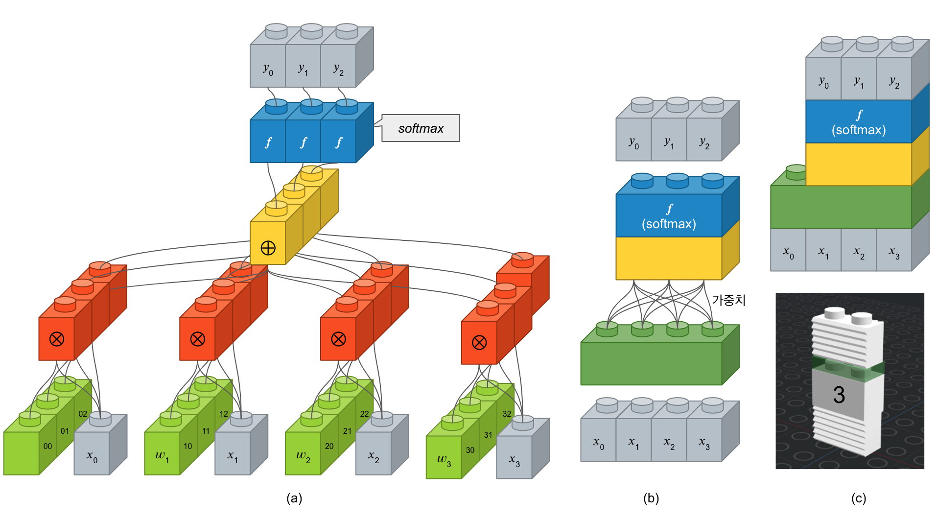
신경망에서 가장 기본적인 요소가 ‘뉴론’입니다. 이러한 뉴론 여러개가 구성된 것이 ‘레이어’이고 레이어가 여러 층으로 쌓여있는 것을 ‘네트워크’라 합니다. 입력 뉴런과 출력 뉴런 간에 연결선을 시냅스라 부르고 이 연결 강도를 ‘가중치’라고 합니다. 아래 그림은 입력 4개에 출력 3개 뉴런을 가진 전결합층을 표한한 것입니다. (a)에서 보면 학습해야할 녹색 가중치 블록이 12개가 있습니다. 이를 좀 더 간단하게 표시한 것이 (b)인데, 여기서는 가중치가 연결선으로만 표시되어 있습니다. (c)는 (b)를 좀 더 간략하게 표시한 것입니다. (c)의 아래 그림을 보면 ‘3’으로 표기되어 있는 데, 이는 출력 뉴런의 수를 표기한 것입니다. 케라스에서는 입력 뉴런 수는 입력에 따라 정해지기 때문에 입력층이 아닌 은닉층에서는 따로 지정할 필요는 없습니다.
여러개의 층을 쌓아보자
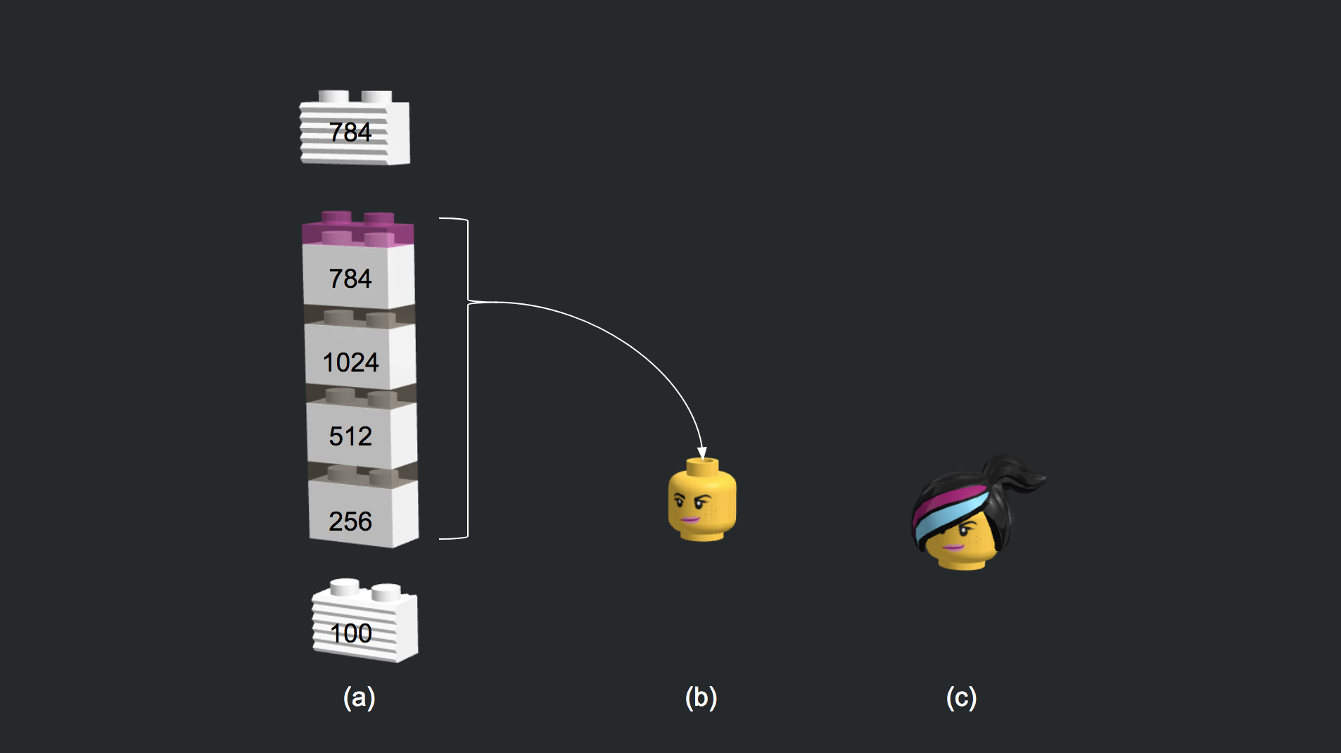
from keras.models import Sequential from keras.layers.core import Dense from keras.layers.advanced_activations import LeakyReLU generator = Sequential() generator.add(Dense(256, input_dim=100)) generator.add(LeakyReLU(0.2)) generator.add(Dense(512)) generator.add(LeakyReLU(0.2)) generator.add(Dense(1024)) generator.add(LeakyReLU(0.2)) generator.add(Dense(784, activation='tanh'))입출력에 대한 설명.
import numpy as np random_latent_vectors = np.random.normal(0, 1, size=[1, 100]) generated_data = generator.predict(random_latent_vectors) generated_images = generated_data.reshape(1, 28, 28)(-0.5, 27.5, 27.5, -0.5)
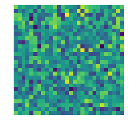
%matplotlib inline import matplotlib.pyplot as plt plt.imshow(generated_images[0], interpolation='nearest') plt.axis('off')import os os.environ["KERAS_BACKEND"] = "tensorflow" import numpy as np from tqdm import tqdm import matplotlib.pyplot as plt from keras.layers import Input from keras.models import Model, Sequential from keras.layers.core import Reshape, Dense, Dropout, Flatten from keras.layers.advanced_activations import LeakyReLU from keras.layers.convolutional import Convolution2D, UpSampling2D from keras.layers.normalization import BatchNormalization from keras.datasets import mnist from keras.optimizers import Adam from keras import backend as K from keras import initializers K.set_image_dim_ordering('th') # Deterministic output. # Tired of seeing the same results every time? Remove the line below. np.random.seed(1000) # The results are a little better when the dimensionality of the random vector is only 10. # The dimensionality has been left at 100 for consistency with other GAN implementations. randomDim = 100 # 1. 데이터셋 생성하기 # Load MNIST data (X_train, y_train), (X_test, y_test) = mnist.load_data() X_train = (X_train.astype(np.float32) - 127.5)/127.5 X_train = X_train.reshape(60000, 784) # 2. 모델 구성하기 # 2.1 생성기 모델 generator = Sequential() generator.add(Dense(256, input_dim=latent_dim)) generator.add(LeakyReLU(0.2)) generator.add(Dense(512)) generator.add(LeakyReLU(0.2)) generator.add(Dense(1024)) generator.add(LeakyReLU(0.2)) generator.add(Dense(784, activation='tanh')) # 2.2 판별기 모델 discriminator = Sequential() discriminator.add(Dense(1024, input_dim=784)) discriminator.add(LeakyReLU(0.2)) discriminator.add(Dropout(0.3)) discriminator.add(Dense(512)) discriminator.add(LeakyReLU(0.2)) discriminator.add(Dropout(0.3)) discriminator.add(Dense(256)) discriminator.add(LeakyReLU(0.2)) discriminator.add(Dropout(0.3)) discriminator.add(Dense(1, activation='sigmoid')) # 2.3 간 모델 ganInput = Input(shape=(randomDim,)) x = generator(ganInput) ganOutput = discriminator(x) gan = Model(inputs=ganInput, outputs=ganOutput) # 3. 모델 학습과정 설정하기 # Optimizer adam = Adam(lr=0.0002, beta_1=0.5) # 3.1 판별기 모델 학습과정 설정 discriminator.compile(loss='binary_crossentropy', optimizer=adam) # 3.2 간 모델 학습과정 설정 discriminator.trainable = False gan.compile(loss='binary_crossentropy', optimizer=adam) dLosses = [] gLosses = [] # Plot the loss from each batch def plotLoss(epoch): plt.figure(figsize=(10, 8)) plt.plot(dLosses, label='Discriminitive loss') plt.plot(gLosses, label='Generative loss') plt.xlabel('Epoch') plt.ylabel('Loss') plt.legend() plt.savefig('./warehouse/simplegan/images/gan_loss_epoch_%d.png' % epoch) # Create a wall of generated MNIST images def plotGeneratedImages(epoch, examples=100, dim=(10, 10), figsize=(10, 10)): noise = np.random.normal(0, 1, size=[examples, randomDim]) generatedImages = generator.predict(noise) generatedImages = generatedImages.reshape(examples, 28, 28) plt.figure(figsize=figsize) for i in range(generatedImages.shape[0]): plt.subplot(dim[0], dim[1], i+1) plt.imshow(generatedImages[i], interpolation='nearest', cmap='gray_r') plt.axis('off') plt.tight_layout() plt.savefig('./warehouse/simplegan/images/gan_generated_image_epoch_%d.png' % epoch) # Save the generator and discriminator networks (and weights) for later use def saveModels(epoch): generator.save('./warehouse/simplegan/models/gan_generator_epoch_%d.h5' % epoch) discriminator.save('./warehouse/simplegan/models/gan_discriminator_epoch_%d.h5' % epoch) def train(epochs=1, batchSize=128): batchCount = X_train.shape[0] / batchSize print 'Epochs:', epochs print 'Batch size:', batchSize print 'Batches per epoch:', batchCount for e in xrange(1, epochs+1): print '-'*15, 'Epoch %d' % e, '-'*15 for _ in tqdm(xrange(batchCount)): # Get a random set of input noise and images noise = np.random.normal(0, 1, size=[batchSize, randomDim]) imageBatch = X_train[np.random.randint(0, X_train.shape[0], size=batchSize)] # Generate fake MNIST images generatedImages = generator.predict(noise) # print np.shape(imageBatch), np.shape(generatedImages) X = np.concatenate([imageBatch, generatedImages]) # Labels for generated and real data yDis = np.zeros(2*batchSize) # One-sided label smoothing yDis[:batchSize] = 0.9 # Train discriminator dloss = discriminator.train_on_batch(X, yDis) # Train generator noise = np.random.normal(0, 1, size=[batchSize, randomDim]) yGen = np.ones(batchSize) gloss = gan.train_on_batch(noise, yGen) # Store loss of most recent batch from this epoch dLosses.append(dloss) gLosses.append(gloss) plotGeneratedImages(e) if e == 1 or e % 20 == 0: saveModels(e) # Plot losses from every epoch plotLoss(e) if __name__ == '__main__': train(200, 128)
사소한 변화를 무시해주는 맥스풀링(Max Pooling) 레이어
컨볼루션 레이어의 출력 이미지에서 주요값만 뽑아 크기가 작은 출력 영상을 만듭니다. 이것은 지역적인 사소한 변화가 영향을 미치지 않도록 합니다.
MaxPooling2D(pool_size=(2, 2))주요 인자는 다음과 같습니다.
- pool_size : 수직, 수평 축소 비율을 지정합니다. (2, 2)이면 출력 영상 크기는 입력 영상 크기의 반으로 줄어듭니다.
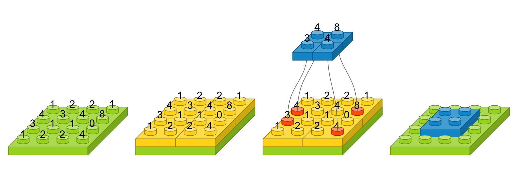
예를 들어, 입력 영상 크기가 4 x 4이고, 풀 크기를 (2, 2)로 했을 때를 도식화하면 다음과 같습니다. 녹색 블록은 입력 영상을 나타내고, 노란색 블록은 풀 크기에 따라 나눈 경계를 표시합니다. 해당 풀에서 가장 큰 값을 선택하여 파란 블록으로 만들면, 그것이 출력 영상이 됩니다. 가장 오른쪽은 맥스풀링 레이어를 약식으로 표시한 것입니다.
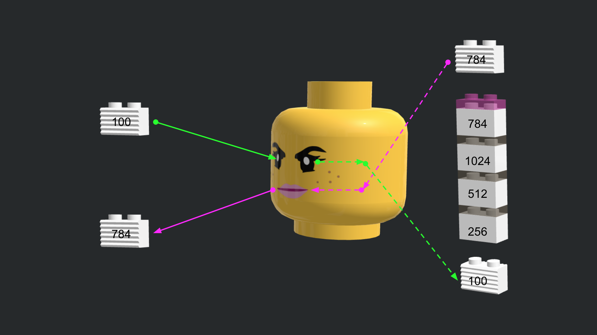
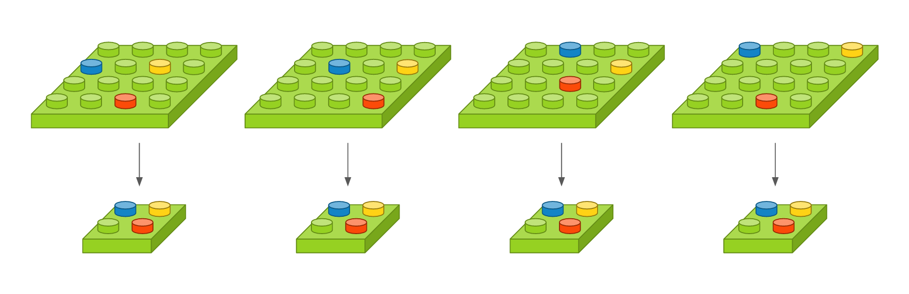
이 레이어는 영상의 작은 변화라던지 사소한 움직임이 특징을 추출할 때 크게 영향을 미치지 않도록 합니다. 영상 내에 특징이 세 개가 있다고 가정했을 때, 아래 그림에서 첫 번째 영상을 기준으로 두 번째 영상은 오른쪽으로 이동하였고, 세 번째 영상은 약간 비틀어 졌고, 네 번째 영상은 조금 확대되었지만, 맥스풀링한 결과는 모두 동일합니다. 얼굴 인식 문제를 예를 들면, 맥스풀링의 역할은 사람마다 눈, 코, 입 위치가 조금씩 다른데 이러한 차이가 사람이라고 인식하는 데 있어서는 큰 영향을 미치지 않게 합니다.
영상을 일차원으로 바꿔주는 플래튼(Flatten) 레이어
CNN에서 컨볼루션 레이어나 맥스풀링 레이어를 반복적으로 거치면 주요 특징만 추출되고, 추출된 주요 특징은 전결합층에 전달되어 학습됩니다. 컨볼루션 레이어나 맥스풀링 레이어는 주로 2차원 자료를 다루지만 전결합층에 전달하기 위해선 1차원 자료로 바꿔줘야 합니다. 이 때 사용되는 것이 플래튼 레이어입니다. 사용 예시는 다음과 같습니다.
Flatten()이전 레이어의 출력 정보를 이용하여 입력 정보를 자동으로 설정되며, 출력 형태는 입력 형태에 따라 자동으로 계산되기 때문에 별도로 사용자가 파라미터를 지정해주지 않아도 됩니다. 크기가 3 x 3인 영상을 1차원으로 변경했을 때는 도식화하면 다음과 같습니다.

한 번 쌓아보기
지금까지 알아본 레이어를 이용해서 간단한 컨볼루션 신경망 모델을 만들어보겠습니다. 먼저 간단한 문제를 정의해봅시다. 손으로 삼각형, 사각형, 원을 손으로 그린 이미지가 있고 이미지 크기가 8 x 8이라고 가정해봅니다. 삼각형, 사각형, 원을 구분하는 3개의 클래스를 분류하는 문제이기 때문에 출력 벡터는 3개여야 합니다. 필요하다고 생각하는 레이어를 구성해봤습니다.

- 컨볼루션 레이어 : 입력 이미지 크기 8 x 8, 입력 이미지 채널 1개, 필터 크기 3 x 3, 필터 수 2개, 경계 타입 ‘same’, 활성화 함수 ‘relu’
- 맥스풀링 레이어 : 풀 크기 2 x 2

- 컨볼루션 레이어 : 입력 이미지 크기 4 x 4, 입력 이미지 채널 2개, 필터 크기 2 x 2, 필터 수 3개, 경계 타입 ‘same’, 활성화 함수 ‘relu’

- 맥스풀링 레이어 : 풀 크기 2 x 2

- 플래튼 레이어

- 댄스 레이어 : 입력 뉴런 수 12개, 출력 뉴런 수 8개, 활성화 함수 ‘relu’

- 댄스 레이어 : 입력 뉴런 수 8개, 출력 뉴런 수 3개, 활성화 함수 ‘softmax’

모든 레이어 블록이 준비되었으니 이를 조합해 봅니다. 입출력 크기만 맞으면 블록 끼우듯이 합치면 됩니다. 참고로 케라스 코드에서는 가장 첫번째 레이어를 제외하고는 입력 형태를 자동으로 계산하므로 이 부분은 신경쓰지 않아도 됩니다. 레이어를 조립하니 간단한 컨볼루션 모델이 생성되었습니다. 이 모델에 이미지를 입력하면, 삼각형, 사각형, 원을 나타내는 벡터가 출력됩니다.

그럼 케라스 코드로 어떻게 구현하는 지 알아봅니다. 먼저 필요한 패키지를 추가하는 과정입니다. 케라스의 레이어는 ‘keras.layers’에 정의되어 있으며, 여기서 필요한 레이어를 추가합니다.
import numpy from keras.models import Sequential from keras.layers import Dense from keras.layers import Flatten from keras.layers.convolutional import Conv2D from keras.layers.convolutional import MaxPooling2D from keras.utils import np_utilsUsing Theano backend.Sequential 모델을 하나 생성한 뒤 위에서 정의한 레이어를 차례차레 추가하면 컨볼루션 모델이 생성됩니다.
model = Sequential() model.add(Conv2D(2, (3, 3), padding='same', activation='relu', input_shape=(8, 8, 1))) model.add(MaxPooling2D(pool_size=(2, 2))) model.add(Conv2D(3, (2, 2), padding='same', activation='relu')) model.add(MaxPooling2D(pool_size=(2, 2))) model.add(Flatten()) model.add(Dense(8, activation='relu')) model.add(Dense(3, activation='softmax'))생성한 모델을 케라스에서 제공하는 함수를 이용하여 가시화 시켜봅니다.
from IPython.display import SVG
from keras.utils.vis_utils import model_to_dot

%matplotlib inline

SVG(model_to_dot(model, show_shapes=True).create(prog='dot', format='svg'))

요약
컨볼루션 신경망 모델에서 사용되는 주요 레이어의 원리와 역할에 대해서 알아보았고 레이어를 조합하여 간단한 컨볼루션 신경망 모델을 만들어봤습니다.
같이 보기
책 소개
[추천사]
- 하용호님, 카카오 데이터사이언티스트 - 뜬구름같은 딥러닝 이론을 블록이라는 손에 잡히는 실체로 만져가며 알 수 있게 하고, 구현의 어려움은 케라스라는 시를 읽듯이 읽어내려 갈 수 있는 라이브러리로 풀어준다.
- 이부일님, (주)인사아트마이닝 대표 - 여행에서도 좋은 가이드가 있으면 여행지에 대한 깊은 이해로 여행이 풍성해지듯이 이 책은 딥러닝이라는 분야를 여행할 사람들에 가장 훌륭한 가이드가 되리라고 자부할 수 있다. 이 책을 통하여 딥러닝에 대해 보지 못했던 것들이 보이고, 듣지 못했던 것들이 들리고, 말하지 못했던 것들이 말해지는 경험을 하게 될 것이다.
- 이활석님, 네이버 클로바팀 - 레고 블럭에 비유하여 누구나 이해할 수 있게 쉽게 설명해 놓은 이 책은 딥러닝의 입문 도서로서 제 역할을 다 하리라 믿습니다.
- 김진중님, 야놀자 Head of STL - 복잡했던 머릿속이 맑고 깨끗해지는 효과가 있습니다.
- 이태영님, 신한은행 디지털 전략부 AI LAB - 기존의 텐서플로우를 활용했던 분들에게 바라볼 수 있는 관점의 전환점을 줄 수 있는 Mild Stone과 같은 책이다.
- 전태균님, 쎄트렉아이 - 케라스의 특징인 단순함, 확장성, 재사용성을 눈으로 쉽게 보여주기 위해 친절하게 정리된 내용이라 생각합니다.
- 유재준님, 카이스트 - 바로 적용해보고 싶지만 어디부터 시작할지 모를 때 최선의 선택입니다.